7 Uses and prediction

DRAFT

Once a volume or biomass model has been fitted, several uses may be made of its predictions. Most commonly, it is used to predict the volume or biomass of trees whose volume or biomass has not been measured. This is prediction in the strictest sense (§ 7.2–7.4). Sometimes, tree volume or biomass will also have been measured in addition to table entry variables. In this case, when a dataset is available independently of that used to fit the model, and which contains both the model’s response variable and its effect variables, this can be used to validate the model (§ 7.1). When validation criteria are applied to the same dataset that served to calibrate the model, we speak of model verification We will not dwell here on model verification as this is already implicit in the analysis of the fitted model’s residuals. Finally, if we are in possession of models that were developed prior to a new fitted model, we may also wish to compare or combine the models (§ 7.5).

Model valid range

Before using a model, we must check that the characteristics of the tree whose volume or biomass we wish to predict fall within the valid range of the model (Rykiel 1996). If a volume or biomass model has been fitted for trees of dbh between \(D_{\min}\) and \(D_{\max}\), in principle it cannot be used to predict the volume or biomass of a tree whose dbh is less than \(D_{\min}\) or more than \(D_{\max}\). The same applies for all model entries. But not all models are subject to the same errors when extrapolating outside their valid range. Power models can generally be extrapolated outside their valid range and still yield reliable results as they are based on a fractal allometric model that is invariant on all scales (Zianis and Mencuccini 2004). By contrast, polynomial models often behave abnormally outside their valid range (e.g. predicting negative values), particularly when using high-order polynomials.

7.1 Validating a model

Validating a model consists in comparing its predictions with observations independent of those used for its fitting (Rykiel 1996). Let (\(Y'_i\), \(X'_{i1}\), \(\ldots\), \(X'_{ip}\)) with \(i=1\), \(\ldots\), \(n'\) be a dataset of observations independent of that used to fit a model \(f\), where \(X'_{i1}\), \(\ldots\), \(X'_{ip}\) are the effect variables and \(Y'_i\) is the response variable, i.e. the volume, biomass or a transform of one of these quantities. Let \[ \hat{Y}'_i=f(X'_{i1},\ \ldots,\ X'_{ip};\hat{\theta}) \] be the predicted value of the response variable for the \(i\)th observation, where \(\hat{\theta}\) are the estimated values of the model’s parameters. The validation consists in comparing the predicted values \(\hat{Y}'_i\) with the observed values \(Y'_i\).

7.1.1 Validation criteria

Several criteria, which are the counterparts of the criteria used to evaluate the quality of model fitting, may be used to compare predictions with observations (Schlaegel 1982; Parresol 1999; Tedeschi 2006), in particular:

• bias: \(\sum_{i=1}^{n'}|Y'_i-\hat{Y}'_i|\)

• sum of squares of the residuals: \(\mathrm{SSE}=\sum_{i=1}^{n'}(Y'_i-\hat{Y}'_i)^2\)

• residual variance: \(s^2=\mathrm{SSE}/(n'-p)\)

• fitted residual error: \(\mathrm{SSE}/(n'-2p)\)

• \(R^2\) of the regression: \(R^2=1-s^2/\mathrm{Var}(Y')\)

• Akaike information criterion: \(\mathrm{AIC}=n'\ln(s^2)+n'\ln(1-p/n')+2p\)

where \(\mathrm{Var}(Y')\) is the empirical variance of \(Y'\) and \(p\) is the number of freely estimated parameters in the model. The first two criteria correspond to two distinct norms of the difference between the vector (\(Y'_1,\ \ldots,\ Y'_{n'}\)) of the observations and the vector (\(\hat{Y}'_1,\ \ldots,\ \hat{Y}'_{n'}\)) of the predictions: norm \(L^1\) for the bias and norm \(L^2\) for the sum of squares. Any other norm is also valid. The last three criteria involve the number of parameters used in the model, and are therefore more appropriate for comparing different models.

7.1.2 Cross validation

If no independent dataset is available, it is tempting to split the calibration dataset into two subsets: one to fit the model, the other to validate the model. Given that volume or biomass datasets are costly, and often fairly small, we do not recommend this practice when constructing volume or biomass tables. By contrast, in this case, we do recommend the use of cross validation (Efron and Tibshirani 1993, chapitre 17).

A “\(K\) fold” cross validation consists in dividing the dataset into \(K\) subsets of approximately equal size and using each subset, one after the other, as validation datasets, with the model being fitted on the \(K-1\) subsets remaining. The “\(K\) fold” cross validation pseudo-algorithm is as follows:

1. Split the dataset \(\mathcal{S}_n\equiv\{(Y_i,\ X_{i1},\ \ldots,\ X_{ip}): i=1,\ \ldots,\ n\}\) into \(K\) data subsets \(\mathcal{S}_n^{(1)},\ \ldots,\ \mathcal{S}_n^{(K)}\) of approximately equal size (i.e. with about \(n/K\) observations in each data subset, totaling \(n\)).

2. For \(k\) from 1 to \(K\):

   1. fit the model on the dataset deprived of its \(k\)th subset, i.e. on \(\mathcal{S}_n\backslash\mathcal{S}_n^{(k)}=\mathcal{S}_n^{(1)} \cup\ldots\cup\mathcal{S}_n^{(k-1)}\cup\mathcal{S}_n^{(k+1)}\cup\ldots\cup\mathcal{S}_n^{(K)}\);
   2. calculate a validation criterion (see  7.1.1) for this fitted model by using the remaining dataset \(\mathcal{S}_n^{(k)}\) as validation dataset; let \(C_k\) be the value of this criterion calculated for \(\mathcal{S}_n^{(k)}\).

3. Calculate the mean \((\sum_{k=1}^KC_k)/K\) of the \(K\) validation criteria calculated.

The fact that there is no overlap between the data used for model fitting and the data used to calculate the validation criterion means that the approach is valid. Cross validation needs more calculations than a simple validation, but has the advantage of making the most of all the observations available for model fitting.

A special case of a “\(K\) fold” cross validation is when \(K\) is equal to the number \(n\) of observations available in the dataset. This method is also called “leave-one-out” cross validation and is conceptually similar to the Jack-knife technique (Efron and Tibshirani 1993). The principle consists in fitting the model on \(n-1\) observations and calculating the residual error for the observation that was left out. It is used when analyzing the residuals to quantify the influence of the observations (and in particular is the basis of the calculation of Cook’s distance, see Saporta 1990).

7.2 Predicting the volume or biomass of a tree

Making a prediction based on model \(f\) consists in using the known values of the effect variables \(X_1,\ \ldots,\ X_p\), to calculate the predicted value \(\hat{Y}\). A prediction does not end with the calculation of \[ \hat{Y}=f(X_1,\ \ldots,\ X_p;\hat{\theta}) \] The estimator \(\hat{\theta}\) of model parameters is a random vector whose distribution stems from the distribution of the observations used to fit the model. Any model prediction \(\hat{Y}\) is therefore itself a random variable whose distribution stems from the distribution of the observations used to fit the model. If we are to express this intrinsic variability of the prediction, we must associate it with an uncertainty indicator such as the standard deviation of the prediction or its 95 % confidence interval.

Several confidence intervals are available depending on whether we are predicting the volume or biomass of a tree selected at random in the stand, or the volume or biomass of the mean tree in the stand. We will now describe in detail the analytical expressions of these confidence intervals for a linear model (§ 7.2.1), then for a non-linear model (§ 7.2.2). We will then present expressions for these confidence intervals that are similar but simpler to compute (§ 7.2.3, before focusing on the case of transformed variables (§ 7.2.4).

7.2.1 Prediction: linear model

Prediction by simple linear regression

Let \(\hat{a}\) be the estimated y-intercept of a linear regression, and \(\hat{b}\) be its estimated slope. The prediction of \(\hat{Y}\) the response variable may be written in two different ways: \[\begin{eqnarray} \hat{Y}&=&\hat{a}+\hat{b}X\tag{7.1}\\ % \hat{Y}&=&\hat{a}+\hat{b}X+\varepsilon\tag{7.2} \end{eqnarray}\] In both cases the expectation of \(\hat{Y}\) is the same as \(\mathrm{E}(\varepsilon)=0\). By contrast, the variance of \(\hat{Y}\) is not the same: it is higher in the second than in the first. These two equations may be interpreted as follows. Let us assume that effect variable \(X\) is dbh and that the response variable \(Y\) is the biomass. The number of trees in the whole forest with a given dbh \(X\) (to within measurements errors) is immeasurably huge. If we were able to measure the biomass of all these trees with the same dbh, we would obtain variable values oscillating around a certain mean value. If we seek to predict this mean biomass (i.e. the mean of all the trees with dbh \(X\)), then equation (7.1) of the prediction is valid. By contrast, if we seek to predict the biomass of a tree selected at random from all the trees with dbh \(X\), then equation (7.2) of the prediction is valid. The variability of the prediction is greater for (7.2) than for (7.1) because here the variability of the mean biomass prediction is supplemented by the differences in biomass between the trees.

This means that two methods can be used to calculate a confidence interval for a prediction. There is a confidence interval for the prediction of the mean of \(Y\), and a confidence interval for the prediction of an individual selected at random from the population in which the mean of \(Y\) was calculated. The second confidence interval is wider than the first.

In the case of a simple linear regression, it can be shown (Saporta 1990, 373–74) that the confidence interval at a significance level of \(\alpha\) for predicting the mean (7.1) is: \[\begin{equation} \hat{a}+\hat{b}X\pm t_{n-2}\ \hat{\sigma}\sqrt{\frac{1}{n}+\frac{(X-\bar{X})^2}{nS_X^2}} \tag{7.3} \end{equation}\] while the confidence interval at a significance level of \(\alpha\) for predicting a tree selected at random (7.2) is: \[\begin{equation} \hat{a}+\hat{b}X\pm t_{n-2}\ \hat{\sigma}\sqrt{1+\frac{1}{n}+\frac{(X-\bar{X})^2}{nS_X^2}} \tag{7.4} \end{equation}\] where \(t_{n-2}\) is the quantile \(1-\alpha/2\) of a Student’s distribution with \(n-2\) degrees of freedom, \(\bar{X}=(\sum_{i=1}^nX_i)/n\) is the mean of the observed values of \(X\) in the dataset that served to fit the model, and \(S_X^2=[\sum_{i=1}^n(X_i-\bar{X})^2]/n\) is the empirical variance of the observed values of \(X\) in the dataset that served to fit the model.

These expressions call for several remarks. The first is that the difference between the bounds of confidence interval (7.4) for a tree selected at random and the bounds of confidence interval (7.3) for the mean tree is approximately \(t_{n-2}\hat{\sigma}\). This difference reflects the difference between equations (7.2) and (7.1), which is due to the residual term \(\varepsilon\) whose estimated standard deviation is \(\hat{\sigma}\).

The second is that the width of the confidence interval is not constant, but varies with \(X\). The confidence interval is narrowest when \(X=\bar{X}\) but widens as \(X\) moves away from \(\bar{X}\).

The third remark is that in order to calculate the confidence interval of a prediction based on a linear regression, we must be in possession of — if not the original data that served to fit the model — at least the mean \(\bar{X}\) of the effect variable and its empirical standard deviation \(S_X\). If the original data that served to fit the model are not available, and the values of \(\bar{X}\) and \(S_X\) have not been documented, we cannot accurately calculate the confidence interval.

Red line 7.1 \(\looparrowright\) Confidence interval of \(\ln(B)\) predicted by \(\ln(D)\)

Let us return to the simple linear regression between \(\ln(B)\) and \(\ln(D)\) that was fitted in red line 6.1. Let m be the object containing the fitted model (see red line 6.1). The confidence intervals may be calculated using the predict command. For example, for a tree with a dbh of 20~cm, the 95 % confidence interval for the mean tree is obtained by the command:

m <- lm(log(Btot) ~ I(log(dbh)), data = dat[dat$Btot > 0,]) ## red line 7
predict(m, newdata = data.frame(dbh = 20), interval = "confidence", level = 0.95)

which yields:

##         fit       lwr       upr
## 1 -1.354183 -1.533487 -1.174879

Thus, the fitted model is \(\ln(B)=\) -1.3541832 with a 95 % confidence interval of -1.5334873 to -1.174879. For a tree with a dbh of 20 cm selected at random, the confidence interval may be obtained by the command:

predict(
    m, newdata = data.frame(dbh = 20), interval = "prediction", level = 0.95
    )

which yields:

##         fit       lwr        upr
## 1 -1.354183 -2.305672 -0.4026948

Figure 7.1 shows the confidence intervals for the entire range of the data.

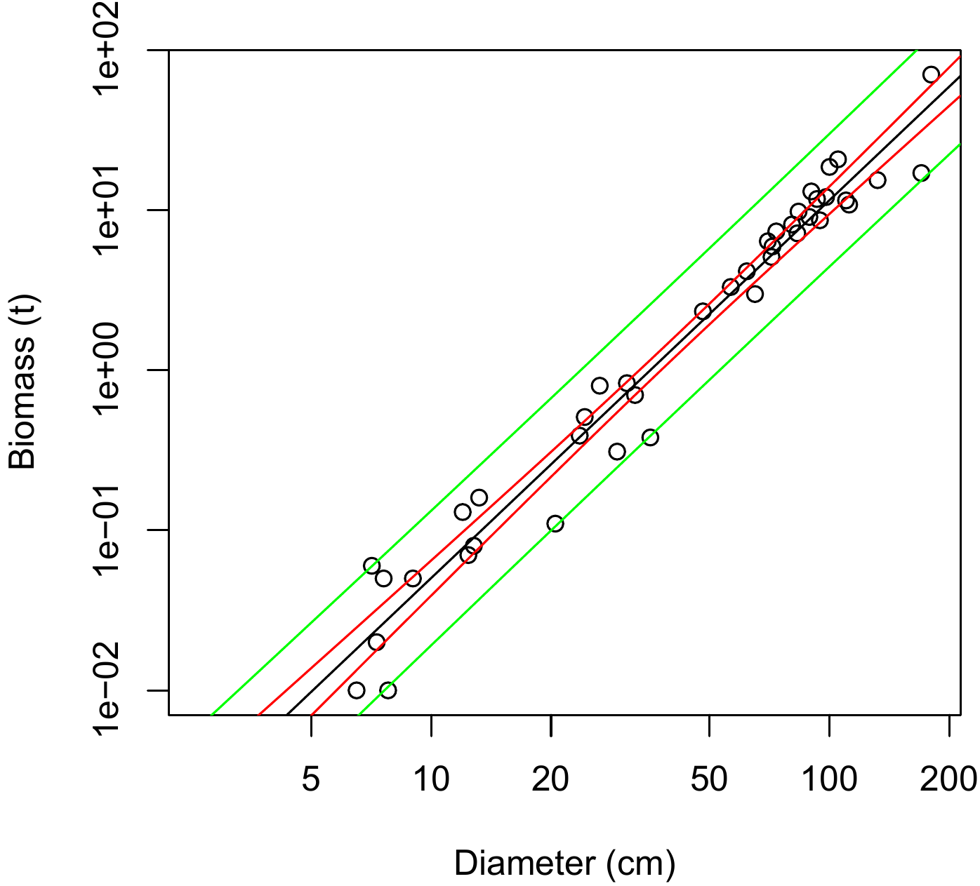
Figure 7.1: Biomass against dbh (on a log scale) for 42 trees measured in Ghana by Henry et al. (2010) (points), prediction (solid line) of the simple linear regression of \(\ln(B)\) against \(\ln(D)\), and confidence intervals of this prediction for a tree selected at random (green line) and for the mean tree (red line).

Prediction by multiple regression

The principles laid down in the case of the linear regression also apply to the multiple regression. The confidence interval can be expressed in two different ways: one for the prediction of the mean tree, the other for the prediction of a tree selected at random.

In the case of a multiple regression with estimated coefficients \(\hat{\mathbf{a}}={}^{\mathrm{t}}[\hat{a}_0,\ \hat{a}_1,\ \hat{a}_2,\ \ldots,\ \hat{a}_p]\), the predicted value \(\hat{Y}\) of the response variable for a tree whose effect variables are \(\mathbf{x}={}^{\mathrm{t}}[1,\ X_1,\ X_2,\ \ldots, X_p]\), is: \[ \hat{Y}={}^{\mathrm{t}}{\mathbf{x}}\ \hat{\mathbf{a}} \] and the confidence interval (with a significance level of \(\alpha\)) of this prediction is (Saporta 1990, 387):

• for the prediction of the mean tree: \[\begin{equation} {}^{\mathrm{t}}{\mathbf{x}}\ \hat{\mathbf{a}}\pm t_{n-p-1}\ \hat{\sigma} \sqrt{{}^{\mathrm{t}}{\mathbf{x}}({}^{\mathrm{t}}{\mathbf{X}}\mathbf{X})^{-1}\mathbf{x}} \tag{7.5} \end{equation}\]

• for the prediction of a tree selected at random: \[\begin{equation} {}^{\mathrm{t}}{\mathbf{x}}\ \hat{\mathbf{a}}\pm t_{n-p-1}\ \hat{\sigma} \sqrt{1+{}^{\mathrm{t}}{\mathbf{x}}({}^{\mathrm{t}}{\mathbf{X}}\mathbf{X})^{-1}\mathbf{x}} \tag{7.6} \end{equation}\]

where \(\mathbf{X}\) is is the design matrix constructed using the data that served to fit the multiple regression. In order to calculate the confidence interval of the predictions, we need to be in possession of — if not the original data that served to fit the model — at least the matrix \(({}^{\mathrm{t}}{\mathbf{X}}\mathbf{X})^{-1}\). It should be noted that the variance of the prediction in the case (7.6) of a tree selected at random is made up of two terms: a term \(\hat{\sigma}^2\) representing the residual error and a term \(\hat{\sigma}^2\;{}^{\mathrm{t}}{\mathbf{x}}({}^{\mathrm{t}}{\mathbf{X}}\mathbf{X})^{-1}\mathbf{x}\) representing the variability induced by the estimation of the model’s coefficients. When estimating the mean tree, the first term disappears, only the second remains.

Red line 7.2 \(\looparrowright\) Confidence interval of \(\ln(B)\) predicted by \(\ln(D)\) and \(\ln(H)\)

Let us return to the multiple linear regression between \(\ln(B)\), \(\ln(D)\) and \(\ln(H)\) that was fitted in red line 6.4. Let m be the object containing the fitted model (see red line 6.4). The confidence intervals may be calculated using the predict command. For example, for a tree with a dbh of 20~cm and a height of 20 m, the 95 % confidence interval for the mean tree is obtained by the command:

m <- lm(log(Btot) ~ I(log(dbh)) + I(log(heig)), data = dat[dat$Btot > 0,])
predict(
    m, newdata = data.frame(dbh = 20, heig = 20), 
    interval = "confidence", level = 0.95
    )

which yields:

##         fit       lwr       upr
## 1 -1.195004 -1.380798 -1.009211

Thus, the model predicts \(\ln(B)=\) -1.1950044 with a 95 % confidence interval of -1.3807983 to -1.0092105. For a tree with a dbh of 20 cm and a height of 20 m selected at random, the confidence interval is obtained by the command:

predict(
    m, newdata = data.frame(dbh = 20, heig = 20), 
    interval = "prediction", level = 0.95
    )

which yields:

##         fit       lwr        upr
## 1 -1.195004 -2.046408 -0.3436006

7.2.2 Prediction: case of a non-linear model

In the general case of a non-linear model as defined by \[ Y=f(X_1,\ \ldots,\ X_p;\theta)+\varepsilon \] where \[ \varepsilon\mathop{\sim}\mathcal{N}(0,\;kX_1^c) \] unlike the case of the linear model, there is no exact explicit expression for the confidence intervals of the predictions. But the \(\delta\)-method can be used to obtain an approximate (and asymptotically exact) expression of these confidence intervals (Serfling 1980). As before, there are two confidence intervals:

• a confidence interval for the prediction of the mean tree: \[\begin{equation} f(X_1,\ \ldots,\ X_p;\hat{\theta})\pm t_{n-q} \sqrt{{}^{\mathrm{t}}{[\mathrm{d}_{\theta}f(\hat{\theta})]}\;\hat{\boldsymbol{\Sigma}}_{\hat{\theta}}\; [\mathrm{d}_{\theta}f(\hat{\theta})]}\tag{7.7} \end{equation}\]

• a confidence interval for the prediction of a tree selected at random: \[\begin{equation} f(X_1,\ \ldots,\ X_p;\hat{\theta})\pm t_{n-q} \sqrt{\hat{k}^2X_1^{2\hat{c}}+ {}^{\mathrm{t}}{[\mathrm{d}_{\theta}f(\hat{\theta})]}\;\hat{\boldsymbol{\Sigma}}_{\hat{\theta}}\; [\mathrm{d}_{\theta}f(\hat{\theta})]}\tag{7.8} \end{equation}\]

where \(q\) is the number of coefficients in the model (i.e. the length of vector \(\theta\)), \(\mathrm{d}_{\theta}f(\hat{\theta})\) is the value in \(\theta=\hat{\theta}\) of the differential of \(f\) respect to model coefficients, and \(\hat{\boldsymbol{\Sigma}}_{\hat{\theta}}\) is an estimation in \(\theta=\hat{\theta}\) of the variance-covariance matrix \(\boldsymbol{\Sigma}_{\theta}\) of the estimator of \(\theta\). The differential of \(f\) with respect to model coefficients is the vector of length \(q\): \[ \mathrm{d}_{\theta}f(\theta)={}^{\mathrm{t}}{\bigg[\bigg(\frac{\partial f(X_1,\ \ldots,\ X_p;\theta)}{\partial\theta_1}\bigg),\; \ldots,\; \bigg(\frac{\partial f(X_1,\ \ldots,\ X_p;\theta)}{\partial\theta_q}\bigg)\bigg]} \] where \(\theta_i\) is the \(i\)th element of vector \(\theta\). If using the estimator of the maximum likelihood of \(\theta\), we can show that asymptotically, when \(n\rightarrow\infty\) (Saporta 1990, 301): \[ \boldsymbol{\Sigma}_{\theta}\ \mathop{\sim}_{n\rightarrow\infty}\ \mathbf{I}_n(\theta)^{-1}=\frac{1}{n}\; \mathbf{I}_1(\theta)^{-1} \] where \(\mathbf{I}_n(\theta)\) is the Fisher information matrix provided by a sample of size \(n\) on the vector of parameters \(\theta\). This Fisher information matrix has \(q\) lines and \(q\) columns and is calculated from the second derivative of the log-likelihood of the sample: \[ \mathbf{I}_n(\theta)=-\mathrm{E}\bigg[\frac{\partial^2\mathcal{L}(\theta)} {\partial\theta^2}\bigg] \] An approximate estimation of the variance-covariance matrix of the parameters is therefore: \[ \hat{\boldsymbol{\Sigma}}_{\hat{\theta}}=-\bigg[\bigg(\frac{\partial^2\mathcal{L}(\theta)} {\partial\theta^2}\bigg)\bigg|_{\theta=\hat{\theta}}\bigg]^{-1} \] In practice, the algorithm that numerically optimizes the log-likelihood of the sample at the same time gives a numerical estimation of the second derivative \((\partial^2\mathcal{L}/\partial\theta^2)\). This provides an immediate numerical estimation of \(\hat{\boldsymbol{\Sigma}}_{\hat{\theta}}\).

As before, the variance of the predictions in the case (7.8) of a tree selected at random is made up of two terms: a term \((\hat{k}X_1^{\hat{c}})^2\) representing the residual error and a term \({}^{\mathrm{t}}{[\mathrm{d}_{\theta}f(\hat{\theta})]}\;\hat{\boldsymbol{\Sigma}}_{\hat{\theta}}\;[\mathrm{d}_{\theta}f(\hat{\theta})]\) representing the variability induced by the estimation of the model’s coefficients. When estimating the mean tree, the first term disappears, only the second remains.

7.2.3 Approximated confidence intervals

The exact calculation of prediction confidence intervals requires information (matrix \(\mathbf{X}\) for a linear model, variance-covariance matrix \(\hat{\boldsymbol{\Sigma}}_{\hat{\theta}}\) for a non-linear model) that is only rarely given in papers on volume or biomass tables. Generally, these papers provide only the number \(n\) of observations used to fit the model and the residual standard deviation \(\hat{\sigma}\) (linear model) or \(\hat{k}\) and \(\hat{c}\) (non-linear model). Sometimes, even this basic information about the fitting is missing. If \(\mathbf{X}\) (linear model) or \(\hat{\boldsymbol{\Sigma}}_{\hat{\theta}}\) (non-linear model) is not provided, it is impossible to use the formulas given above to calculate confidence intervals. In this case we must use an approximate method.

Residual error alone

Very often, only the residual standard deviation \(\hat{\sigma}\) (linear model) or \(\hat{k}\) and \(\hat{c}\) (non-linear model) is given. In this case, an approximate confidence interval with a significance level of \(\alpha\) may be determined:

• in the case of a linear regression: \[\begin{equation} (a_0+a_1X_1+\ldots+a_pX_p)\pm q_{1-\alpha/2}\ \hat{\sigma} \tag{7.9} \end{equation}\]

• in the case of a non-linear model: \[\begin{equation} f(X_1,\ \ldots,\ X_p;\theta)\pm q_{1-\alpha/2}\ \hat{k}X_1^{\hat{c}} \tag{7.10} \end{equation}\]

where \(q_{1-\alpha/2}\) is the quantile \(1-\alpha/2\) of the standard normal distribution. This confidence interval is a direct retranscription of the relation \(Y=a_0+a_1X_1+\ldots+a_pX_p+\varepsilon\) with \(\varepsilon\sim\mathcal{N}(0,\ \hat{\sigma})\) (linear case) or \(Y=f(X_1,\ \ldots,\ X_p;\theta)+\varepsilon\) with \(\varepsilon\sim\mathcal{N}(0,\ \hat{k}X_1^{\hat{c}})\) (non-linear case), where we have deliberately written the model’s coefficients without a circumflex to underline that these are fixed values. These relations therefore assume implicatively that the model’s coefficients are exactly known and that the only source of variability is the residual error. In other words, these approximate confidence intervals may be interpreted as follows: these confidence intervals (7.9) (linear case) and (7.10) (non-linear case) are those that would be obtained for the prediction of a tree selected at random if sample size was infinite. This is confirmed when \(n\rightarrow\infty\), \(t_{n-p-1}\) tends toward \(q_{1-\alpha/2}\) and the matrix \(({}^{\mathrm{t}}{\mathbf{X}}\mathbf{X})^{-1}\) in (7.6) tends toward the null matrix (whose coefficients are all zero). Thus, confidence interval (7.9) is indeed the bound of confidence interval (7.6) when \(n\rightarrow\infty\). The same may be said of (7.8) and (7.10).

Confidence interval for the mean tree

If an estimation \(\hat{\boldsymbol{\Sigma}}\) is given of the variance-covariance matrix of the parameters, a confidence interval at a significance level of \(\alpha\) for the prediction of the mean tree corresponds to:

• for a linear model: \[\begin{equation} (\hat{a}_0+\hat{a}_1X_1+\ldots+\hat{a}_pX_p)\pm q_{1-\alpha/2}\sqrt{{}^{\mathrm{t}}{\mathbf{x}}\hat{\boldsymbol{\Sigma}}\mathbf{x}} \tag{7.11} \end{equation}\] where \(\mathbf{x}\) is the vector \({}^{\mathrm{t}}{[X_1,\ \ldots,\ X_p]}\),

• for a non-linear model: \[\begin{equation} f(X_1,\ \ldots,\ X_p;\hat{\theta})\pm q_{1-\alpha/2} \sqrt{{}^{\mathrm{t}}{[\mathrm{d}_{\theta}f(\hat{\theta})]}\;\hat{\boldsymbol{\Sigma}}\; [\mathrm{d}_{\theta}f(\hat{\theta})]}\tag{7.12} \end{equation}\]

These confidence intervals consider that all the prediction’s variability stems from the estimation of the model’s coefficients. Also, these confidence intervals are a direct retranscription of the fact that the model’s coefficients follow a multinormal distribution whose mean is their true value and that has a variance-covariance matrix \(\hat{\boldsymbol{\Sigma}}\) for in the linear case, if \(\hat{\mathbf{a}}={}^{\mathrm{t}}{[\hat{a}_1,\ \ldots,\ \hat{a}_p]}\) follows a multinormal distribution of mean \({}^{\mathrm{t}}{[a_1,\ \ldots,\ a_p]}\) and variance-covariance matrix \(\hat{\boldsymbol{\Sigma}}\), then the linear combination \({}^{\mathrm{t}}{\mathbf{x}}\ \hat{\mathbf{a}}\) follows a normal distribution of mean \({}^{\mathrm{t}}{\mathbf{x}}\ \mathbf{a}\) and variance \({}^{\mathrm{t}}{\mathbf{x}}\hat{\boldsymbol{\Sigma}}\mathbf{x}\) (Saporta 1990, 85).

In the case of a linear model, we can show that the variance-covariance matrix of the estimator of the model’s coefficients is (Saporta 1990, 380): \(\boldsymbol{\Sigma}=\sigma^2({}^{\mathrm{t}}{\mathbf{X}}\mathbf{X})^{-1}\). Thus, an estimation of this variance-covariance matrix is: \(\hat{\boldsymbol{\Sigma}}=\hat{\sigma}^2({}^{\mathrm{t}}{\mathbf{X}}\mathbf{X})^{-1}\). By integrating this expression in (7.11), we create an expression similar to (7.5). Similarly, in the non-linear case, confidence interval (7.12) is an approximation of (7.7).

In the non-linear case (7.12), if we want to avoid calculating the partial derivatives of \(f\), we could use the Monte Carlo method. This method is based on a simulation that consists in making \(Q\) samplings of coefficients \(\theta\) in accordance with a multinormal distribution of mean \(\hat{\theta}\) and variance-covariance matrix \(\hat{\boldsymbol{\Sigma}}\), calculating the prediction for each of the simulated values, then calculating the empirical confidence interval of these \(Q\) predictions. This method is known in the literature as providing “population prediction intervals” (Bolker 2008; Paine et al. 2012). The pseudo-algorithm is as follows:

1. For \(k\) of \(1\) to \(Q\): a. draw a vector \(\hat{\theta}^{(k)}\) following a multinormal distribution of mean \(\hat{\theta}\) and variance-covariance matrix \(\hat{\boldsymbol{\Sigma}}\); b. calculate the prediction \(\hat{Y}^{(k)}=f(X_1,\ \ldots,\ X_p;\hat{\theta}^{(k)})\).
2. The confidence interval of the prediction is the empirical confidence interval of the \(Q\) values \(\hat{Y}^{(1)},\ \ldots,\ \hat{Y}^{(Q)}\).

Very often we do not know the variance-covariance matrix \(\hat{\boldsymbol{\Sigma}}\), but we do have an estimation of the standard deviations of the coefficients. Let \(\mathrm{Var}(\hat{a}_i)=\Sigma_i\) (linear case) or \(\mathrm{Var}(\hat{\theta}_i)=\Sigma_i\) (non-linear case) be the variance of the model’s \(i\)th coefficient. In this case we will ignore the correlation between the model’s coefficients and will approximate the variance-covariance matrix of the coefficients by a diagonal matrix: \[ \hat{\boldsymbol{\Sigma}}\approx\left[ \begin{array}{ccc} \hat{\Sigma}_1 & & \mathbf{0}\\ % & \ddots & \\ % \mathbf{0} & & \hat{\Sigma}_p\\ % \end{array} \right] \]

Confidence interval for a tree selected at random

The error resulting from the estimation of the model’s coefficients, as described in the last section, can be cumulated with the residual error described in the section before last, in order to construct a prediction confidence interval for a tree selected at random. These are the variances of the predictions that are added one to the other. The confidence interval with a significance level of \(\alpha\) is therefore:

• for a linear model: \[ (\hat{a}_0+\hat{a}_1X_1+\ldots+\hat{a}_pX_p)\pm q_{1-\alpha/2}\sqrt{\hat{\sigma}^2+{}^{\mathrm{t}}{\mathbf{x}}\hat{\boldsymbol{\Sigma}}\mathbf{x}} \] which is an approximation of (7.6),

• for a non-linear model: \[ f(X_1,\ \ldots,\ X_p;\hat{\theta})\pm q_{1-\alpha/2} \sqrt{\hat{k}^2X_1^{2\hat{c}}+{}^{\mathrm{t}}{[\mathrm{d}_{\theta}f(\hat{\theta})]}\; \hat{\boldsymbol{\Sigma}}\; [\mathrm{d}_{\theta}f(\hat{\theta})]} \] which is an approximation of (7.8).

As before, if we want to avoid a great many calculations, we could employ the Monte Carlo method, using the following pseudo-algorithm:

1. For \(k\) of \(1\) to \(Q\): a. draw a vector \(\hat{\theta}^{(k)}\) following a multinormal distribution of mean \(\hat{\theta}\) and variance-covariance matrix \(\hat{\boldsymbol{\Sigma}}\); a. draw a residual \(\hat{\varepsilon}^{(k)}\) following a centered normal distribution of standard deviation \(\hat{\sigma}\) (linear case) or \(\hat{k}X_1^{\hat{c}}\) (non-linear case); a. calculate the prediction \(\hat{Y}^{(k)}=f(X_1,\ \ldots,\ X_p;\hat{\theta}^{(k)})+\hat{\varepsilon}^{(k)}\).

2. The confidence interval of the prediction is the empirical confidence interval of the \(Q\) values \(\hat{Y}^{(1)},\ \ldots,\ \hat{Y}^{(Q)}\).

Confidence interval with measurement uncertainties

Fitting volume and biomass models assumes that the effect variables \(X_1,\ \ldots,\ X_p\) are known exactly. In actual fact, this hypothesis is only an approximation as these variables are measured and are therefore subject to measurement error. Warning: measurement error should not be confused with the residual error of the response variable: the first is related to the measuring instrument and in principle may be rendered as small as we wish by using increasingly precise measuring instruments. The second reflects the intrinsic biological variability between individuals. We can take account of the impact of measurement error on the prediction by including it in the prediction confidence interval. Thus, the effect variables \(X_1,\ \ldots,\ X_p\) are no longer considered as fixed, but as being contained within a distribution. Typically, to predict the volume or biomass of a tree with characteristics \(X_1,\ \ldots,\ X_p\), we will consider that the \(i\)th characteristic is distributed according to a normal distribution of mean \(X_i\) and standard deviation \(\tau_i\). Typically, if \(X_i\) is a dbh, then \(\tau_i\) will be 3–5~mm; if \(X_i\) is a height, \(\tau_i\) will be 3 % of \(X_i\) for \(X_i\leq15\)~m and 1~m for \(X_i>15\)~m.

It is difficult to calculate an explicit expression for the prediction confidence interval when the effect variables are considered to be random since this means we must calculate the variances of the products of these random variables, some of which are correlated one with the other. The \(\delta\)-method offers an approximate analytical solution (Serfling 1980). Or, more simply, we can again use a Monte Carlo method. In this case, the pseudo-algorithm becomes:

1. For \(k\) of \(1\) to \(Q\): a. for \(i\) of 1 to \(p\), draw \(\hat{X}_i^{(k)}\) following a normal distribution of mean \(X_i\) and standard deviation \(\tau_i\); a. draw a vector \(\hat{\theta}^{(k)}\) following a multinormal distribution of mean \(\hat{\theta}\) and variance-covariance matrix \(\hat{\boldsymbol{\Sigma}}\); a. draw a residual \(\hat{\varepsilon}^{(k)}\) following a centered normal distribution of standard deviation \(\hat{\sigma}\) (linear case) or \(\hat{k}X_1^{\hat{c}}\) (non-linear case); a. calculate the prediction \(\hat{Y}^{(k)}=f(\hat{X}_1^{(k)},\ \ldots,\ \hat{X}_p^{(k)}; \hat{\theta}^{(k)})+\hat{\varepsilon}^{(k)}\).

2. The confidence interval of the prediction is the empirical confidence interval of the \(Q\) values \(\hat{Y}^{(1)},\ \ldots,\ \hat{Y}^{(Q)}\).

This confidence interval corresponds to the prediction for a tree selected at random. To obtain the confidence interval for the mean tree, simply apply the same pseudo-algorithm but replaced step (c) by:

1.   a. (\(\ldots\)) a. (\(\ldots\)) a. with \(\hat{\varepsilon}^{(k)}=0\); a. (\(\ldots\))

7.2.4 Inverse variables transformation

We saw in section 6.1.5 how a variable transformation can render linear a model that initially did not satisfy the hypotheses of the linear model. Variable transformation affects both the mean and the residual error. The same may be said of the inverse transformation, with implications on the calculation of prediction expectation. The log transformation is that most commonly used, but other types of transformation are also available.

Log transformation

Let us first consider the case of the log transformation of volume or biomass values, which is by far the most common case for volume and biomass models. Let us assume that a log transformation has been applied to biomass \(B\) to fit a linear model using effect variables \(X_1,\ \ldots,\ X_p\): \[\begin{equation} Y=\ln(B)=a_0+a_1X_1+\ldots+a_pX_p+\varepsilon\tag{7.13} \end{equation}\] where \[ \varepsilon\mathop{\sim}_{\mathrm{i.i.d.}}\mathcal{N}(0,\ \sigma) \] This is equivalent to saying that \(\ln(B)\) follows a normal distribution of mean \(a_0+a_1X_1+\ldots+a_pX_p\) and standard deviation \(\sigma\) or of saying, by definition, that \(B\) follows a log-normal distribution of parameters \(a_0+a_1X_1+\ldots+a_pX_p\) and \(\sigma\). The expectation of this log-normal distribution is: \[ \mbox{E}(B)=\exp\Big(a_0+a_1X_1+\ldots+a_pX_p+\frac{\sigma^2}{2}\Big) \] Compared to the inverse model of (7.13) which corresponds to \(B=\exp(a_0+a_1X_1+\ldots+a_pX_p)\), the inverse transformation of the residual error introduces bias into the prediction which can be corrected by multiplying the prediction \(\exp(a_0+a_1X_1+\ldots+a_pX_p)\) by an correction factor (Parresol 1999): \[\begin{equation} \mathrm{CF}=\exp\Big(\frac{\hat{\sigma}^2}{2}\Big)\tag{7.14} \end{equation}\] We must however take care as the biomass models reported in the literature, and fitted after log transformation of the biomass, sometimes include this factor and sometimes do not.

If the decimal \(\log_{10}\) has been used for variable transformation rather than the natural log, the correction factor is: \[ \mathrm{CF}=\exp\Big[\frac{(\hat{\sigma}\ln 10)^2}{2}\Big]\approx \exp\Big(\frac{\hat{\sigma}^2}{0.3772}\Big) \]

Red line 7.3 \(\looparrowright\) Correction factor for predicted biomass

Let us return to the biomass model in red line 6.25 fitted by multiple regression on log-transformed data: \[ \ln(B)=-8.38900+0.85715\ln(D^2H)+0.72864\ln(\rho) \] If we consider the starting data but use the exponential function (without taking account of the correction factor), we obtain an under-estimated prediction: \(B=\exp(-8.38900)\times(D^H)^{0.85715}\rho^{0.72864}=2.274\times10^{-4}(D^2H)^{0.85715}\rho^{0.72864}\). Let m be the object containing the fitted model (red line 6.25. The adjustment factor \(\mathrm{CF}=\exp(\hat{\sigma}^2/2)\) is obtained by the command:

dm <- tapply(dat$dens, dat$species, mean)
dat <- cbind(dat, dmoy = dm[as.character(dat$species)])
m <- lm(
    formula = log(Btot) ~ I(log(dbh^2 * heig)) + I(log(dmoy)), 
    data = dat[dat$Btot> 0 ,]
    )
exp(summary(m)$sigma^2 / 2)

and here is 1.0610348. The correct model is therefore: \(B=2.412\times10^{-4}(D^2H)^{0.85715}\rho^{0.72864}\).

Any transformation

In the general case, let \(\psi\) be a variable transformation of the biomass (or volume) such that the response variable \(Y=\psi(B)\) may be predicted by a linear regression against the effect variables \(X_1,\ \ldots,\ X_p\). We shall assume that \(\psi\) is derivable and invertible. As \(\psi(B)\) follows a normal distribution of mean \(a_0+a_1X_1+\ldots+a_pX_p\) and standard deviation \(\sigma\), \(B=\psi^{-1}[\psi(B)]\) has an expectation of (Saporta 1990, 26): \[\begin{equation} \mathrm{E}(B)=\int\psi^{-1}(x)\;\phi(x)\;\mathrm{d}x\tag{7.15} \end{equation}\] where \(\phi\) is the probability density of the normal distribution of mean \(a_0+a_1X_1+\ldots+a_pX_p\) and standard deviation \(\sigma\). This expectation is generally different from \(\psi^{-1}(a_0+a_1X_1+\ldots +a_pX_p)\): the variable transformation induces prediction bias when we return to the starting variable by inverse transformation. The drawback of formula (7.15) is that it requires the calculation of an integral.

When the residual standard deviation \(\sigma\) is small, the \(\delta\)-method (Serfling 1980) provides an approximate expression of this prediction bias: \[\begin{eqnarray*} \mathrm{E}(\mathrm{B}) &\simeq& \psi^{-1}[\mathrm{E}(Y)]+\frac{1}{2}\mathrm{Var}(Y)\; (\psi^{-1})"[\mathrm{E}(Y)] \\ &\simeq& \psi^{-1}(a_0+a_1X_1+\ldots+a_pX_p)+\frac{\sigma^2}{2}\; (\psi^{-1})"(a_0+a_1X_1+\ldots+a_pX_p) \end{eqnarray*}\]

“Smearing” estimation

The “smearing” estimation method is a nonparametric method used to correct prediction bias when an inverse transformation is used on the response variable of a linear model (Duan 1983; Taylor 1986; Manning and Mullahy 2001). Given that we can rewrite biomass (or volume) expectation equation (7.15) as: \[\begin{eqnarray*} \mathrm{E}(B) &=& \int\psi^{-1}(x)\;\phi_0(x-a_0-a_1X1-\ldots-a_pX_p)\;\mathrm{d}x \\ &=& \int\psi^{-1}(x+a_0+a_1X1+\ldots+a_pX_p)\;\mathrm{d}\Phi_0(x) \end{eqnarray*}\] where \(\phi_0\) (respectively \(\Phi_0\)) is the probability density (respectively the distribution function) of the centered normal distribution of standard deviation \(\sigma\), the smearing method consists in replacing \(\Phi_0\) by the empirical distribution function of the residuals from model fitting, i.e.: \[\begin{eqnarray*} B_{\mathrm{smearing}} &=& \int\psi^{-1}(x+a_0+a_1X_1+\ldots+a_pX_p)\times\frac{1}{n}\sum_{i=1}^n\delta (x-\hat{\varepsilon}_i)\ \mathrm{d}x \\ &=& \frac{1}{n}\sum_{i=1}^n\psi^{-1}(a_0+a_1X_1+\ldots+a_pX_p+ \hat{\varepsilon}_i) \end{eqnarray*}\] where \(\delta\) is Dirac’s function with zero mass and \(\hat{\varepsilon}_i\) is the residual of the fitted model for the \(i\)th observation. This method of correcting the prediction bias has the advantage of being both very general and easy to calculate. It has the drawback that the residuals \(\hat{\varepsilon}_i\) of model fitting need to be known. This is not a problem when you yourself fit a model to the data, but is a problem when using published volume or biomass tables that are not accompanied by the residuals.

In the particular case of the log transformation, \(\psi^{-1}\) is the exponential function, and therefore the smearing estimation of the biomass corresponds to: \(\exp(a_0+a_1X_1+\ldots+a_pX_p)\times\mathrm{CF}_{\mathrm{smearing}}\), where the smearing correction factor is: \[ \mathrm{CF}_{\mathrm{smearing}}=\frac{1}{n}\sum_{i=1}^n\exp(\hat{\varepsilon}_i) \] Given that \(\hat{\sigma}^2=(\sum_{i=1}^n\hat{\varepsilon}_i^2)/(n-p-1)\), the smearing correction factor is different from correction factor (7.14). But, on condition that \(\hat{\sigma}\rightarrow0\), the two adjustment coefficients are equivalent.

Red line 7.4 \(\looparrowright\) “Smearing” estimation of biomass

Let us again return to the biomass model in red line 6.25 fitted by multiple regression on log-transformed data: \[ \ln(B)=-8.38900+0.85715\ln(D^2H)+0.72864\ln(\rho) \] The smearing correction factor may be obtained by the command:

mean(exp(residuals(m)))

where m is the object containing the fitted model, and in this example is 1.0598586. By way of a comparison, the previously calculated correction factor (red line 7.3) was 1.061035.

7.3 Predicting the volume or biomass of a stand

If we want to predict the volume or biomass of a stand using biomass tables, we cannot measure model entries for all the trees in the stand, only for a sample. The volume or biomass of the trees in this sample will be calculated using the model, then extrapolated to the entire stand. Predicting the volume or biomass of a stand therefore includes two sources of variability: one related to the model’s individual prediction, the other to the sampling of the trees in the stand. If we rigorously take account of these two sources of variability when making predictions on a stand scale, this will cause complex double sampling problems as mentioned in sections 2.1.2 and 2.3 (Parresol 1999).

The problem is slightly less complex when the sample of trees used to construct the model is independent of the sample of trees in which the entries were measured. In this case we can consider that the prediction error stemming from the model is independent of the sampling error. Let us assume that \(n\) sampling plots of unit area \(A\) were selected in a stand whose total area is \(\mathcal{A}\). Let \(N_i\) be the number of trees found in the \(i\)th plot (\(i=1,\ \ldots,\ n\)) and let \(X_{ij1},\ \ldots,\ X_{ijp}\) be the \(p\) effect variables measured on the \(j\)th tree of the \(i\)th plot (\(j=1,\ \ldots,\ N_i\)). Cunia (1965); Cunia (1987d) considered the particular case where biomass is predicted by multiple regression based on the \(p\) effect variables. The estimation of stand biomass is in this case: \[\begin{eqnarray*} \hat{B} &=& \frac{\mathcal{A}}{n}\sum_{i=1}^n\frac{1}{A}\sum_{j=1}^{N_i} (\hat{a}_0+\hat{a}_1X_{ij1}+\ldots+\hat{a}_pX_{ijp}) \\ &=& \hat{a}_0\Big(\frac{\mathcal{A}}{nA}\sum_{i=1}^nN_i\Big) +\hat{a}_1\Big(\frac{\mathcal{A}}{nA}\sum_{i=1}^n\sum_{j=1}^{N_i}X_{ij1}\Big) +\ldots+\hat{a}_p\Big(\frac{\mathcal{A}}{nA}\sum_{i=1}^n\sum_{j=1}^{N_i}X_{ijp}\Big) \end{eqnarray*}\] where \(\hat{a}_0,\ \ldots,\ \hat{a}_p\) are the estimated coefficients of the regression. If \(X^{\star}_0=(\mathcal{A}/nA)\sum_{i=1}^nN_i\) and for each \(k=1,\ \ldots,\ p\), \[ X^{\star}_k=\frac{\mathcal{A}}{nA}\sum_{i=1}^n\sum_{j=1}^{N_i}X_{ijk} \] The estimated biomass of the stand is therefore \[ \hat{B}=\hat{a}_0X^{\star}_0+\hat{a}_1X^{\star}_1+\ldots+\hat{a}_pX^{\star}_p \] Interestingly, the variability of \(\hat{\mathbf{a}}={}^{\mathrm{t}}[\hat{a}_0,\ \ldots,\ \hat{a}_p]\) depends entirely on model fitting, not on stand sampling, while on the other hand, the variability of \(\mathbf{x}={}^{\mathrm{t}}[X^{\star}_0,\ \ldots,\ X^{\star}_p]\) depends entirely on the sampling, not on the model. Given that these two errors are independent, \[ \mathrm{E}(\hat{B})=\mathrm{E}({}^{\mathrm{t}}{\hat{\mathbf{a}}}\mathbf{x})={}^{\mathrm{t}}{\mathrm{E}(\hat{\mathbf{a}})}\ \mathrm{E}(\mathbf{x}) \] and \[ \mathrm{Var}(\hat{B})={}^{\mathrm{t}}{\mathbf{a}}\boldsymbol{\Sigma}_{\mathbf{x}} \mathbf{a}+{}^{\mathrm{t}}{\mathbf{x}}\boldsymbol{\Sigma}_{\mathbf{a}}\mathbf{x} \] where \(\boldsymbol{\Sigma}_{\mathbf{a}}\) is the \((p+1)\times(p+1)\) variance-covariance matrix of the model’s coefficients while \(\boldsymbol{\Sigma}_{\mathbf{x}}\) is the \((p+1)\times(p+1)\) variance-covariance matrix of the sample of \(\mathbf{x}\). The first matrix is derived from model fitting whereas the second is derived from stand sampling. Thus, the error for the biomass prediction of a stand is the sum of these two terms, one of which is related to the prediction error of the model and the other to stand sampling error.

More generally, the principle is exactly the same as when we considered in section Confidence interval with measurement uncertainties, an uncertainty related to the measurement of the effect variables \(X_1,\ \ldots,\ X_p\). A measurement error is not of the same nature as a sampling error. But from a mathematical standpoint, the calculations are the same: in both cases this means considering that the effect variables \(X_1,\ \ldots,\ X_p\) are random, not fixed. We may therefore, in this general case, use a Monte Carlo method to estimate stand biomass. The pseudo-algorithm of this Monte Carlo method is the same as that used previously :

1. For \(k\) from \(1\) to \(Q\), where \(Q\) is the number of Monte Carlo iterations:
   • 1.1. for \(i\) from 1 to \(p\), draw \(\hat{X}_i^{(k)}\) following a distribution corresponding to the variability of the stand sample (this distribution depends on the type of sampling conducted, the size and number of plots inventoried, etc.);
   • 1.2. draw a vector \(\hat{\theta}^{(k)}\) following a multinormal distribution of mean \(\hat{\theta}\) and variance-covariance matrix \(\hat{\boldsymbol{\Sigma}}\);
   • 1.3. calculate the prediction \(\hat{Y}^{(k)}=f(\hat{X}_1^{(k)},\ \ldots,\ \hat{X}_p^{(k)};\hat{\theta}^{(k)})\).
2. The confidence interval of the prediction is the empirical confidence interval of the \(Q\) values \(\hat{Y}^{(1)}\), \(\ldots\), \(\hat{Y}^{(Q)}\).

7.4 Expanding and converting volume and biomass models

It may happen that we have a model which predicts a variable that is not exactly the one we need, but is closely related to it. For example, we may have a model that predicts the dry biomass of the trunk, but we are looking to predict the total above-ground biomass of the tree. Or, we may have a model that predicts the volume of the trunk, but we are looking to predict its dry biomass. Rather than deciding not to use a model simply because it does not give us exactly what we want, we can use it by default and adjust it using a factor. We can use conversion factors to convert volume to biomass (and vice versa), expansion factors to extrapolate a part to the whole, or combinations of the two. Using this approach Henry et al. (2011) put forward three methods to obtain the total biomass:

• The biomass of the trunk is the product of its volume and specific wood density \(\rho\);
• above-ground biomass is the product of trunk biomass and a biomass expansion factor (BEF);
• above-ground biomass is the product of trunk volume and a biomass expansion and conversion factor (BCEF = BEF\(\times\rho\)).

Tables of these different conversion and expansion factors are available. These values are often very variable as they implicitly include difference sources of variability. Although the default table may be very precise, we often loose the benefit of this precision when using an expansion or correction factor as the prediction error cumulates all the sources of error involved in its calculation.

If we have a table that uses height as entry value, but do not have any height information, we may use a corollary model that predicts height from the entry values we do have (typically a height-dbh relation). Like for conversion and expansion factors, this introduces an additional source of error.

7.5 Arbitrating between different models

If we want to predict the volume or biomass of given trees, we often have a choice between different models. For instance, several models may have been fitted in different places for a given species. Or we may have a local model and a pan-tropical model. Arbitrating between the different models available is not always an easy task (Henry et al. 2011). For example, should we choose a specific, local model fitted using little data (and therefore unbiased a priori but with high prediction variability) or a pan-tropical, multispecific model fitted with a host of data (therefore potentially biased but with low prediction variability)? This shows how many criteria are potentially involved when making a choice: model quality (the range of its validity, its capacity to extrapolate predictions, etc.), its specificity (with local, monospecific models at one extreme and pan-tropical, multispecific models at the other), the size of the dataset used for model fitting (and therefore implicitly the variability of its predictions). Arbitrating between different models should not be confused with model selection, as described in section 6.3.2 for when selecting models their coefficients are not yet known, and when we estimate these coefficients we are looking for the model that best fits the data. When arbitrating between models we are dealing with models already fitted and whose coefficients are known.

Arbitration between different models often takes place without any biomass or volume data. But the case we will focus on here is when we have a reference dataset \(\mathcal{S}_n\), with \(n\) observations of the response variable (volume of biomass) and the effect variables.

7.5.1 Comparing using validation criteria

When we have a dataset \(\mathcal{S}_n\), we can compare the different models available on the basis of the validation criteria described in section 7.1.1, by using \(\mathcal{S}_n\) as the validation dataset. Given that the models do not necessarily have the same number \(p\) of parameters, and in line with the parsimony principle, we should prefer the validation criteria that depend on \(p\) in such a manner as to penalize those models with many parameters.

When comparing a particular, supposedly “best” candidate model with different competitors, we can compare its predictions with those of its competitors. To do this we look to see whether or not the predictions made by its competitors are contained within the confidence interval at a significance level of \(\alpha\) of the candidate model.

7.5.2 Choosing a model

A model may be chosen with respect to a “true” model \(f\) that although unknown may be assumed to exist. Let \(M\) be the number of models available. Let us note as \(\hat{f}_m\) the function of the \(p\) effect variables that predicts volume or biomass based on the \(m\)th model. This function is random as it depends on coefficients that are estimated and therefore have their own distribution. The distribution of \(\hat{f}_m\) therefore describes the variability of the predictions based on the model \(m\), as described in section 7.2. The \(M\) models may have very different forms: the \(\hat{f}_1\) model may correspond to a power function, the \(\hat{f}_2\) model to a polynomial function, etc. We will also assume that there is a function \(f\) of the \(p\) effect variables that describes the “true” relation between the response variable (volume or biomass) and these effect variables. We do not know this “true” relation. We do not know what form it has. But each of the \(M\) models may be considered to be an approximation of the “true” relation \(f\).

In the models selection theory (Massart 2007), the difference between the relation \(f\) and a model \(\hat{f}_m\) is quantified by a function \(\gamma\) that we call the loss function. For example, the loss function may be the norm \(L^2\) of the difference between \(f\) and \(\hat{f}_m\): \[ \gamma(f,\ \hat{f}_m)=\int_{x_1}\ldots\int_{x_p} [f(x_1,\ \ldots,\ x_p)-\hat{f}_m(x_1,\ \ldots,\ x_p)]^2 \ \mathrm{d}x_1\ldots\mathrm{d}x_p \] The expectation of the loss with respect to the distribution of \(\hat{f}_m\) is called the risk (written \(R\)) i.e. when integrating on the variability of model predictions: \[ R=\mathrm{E}[\gamma(f,\ \hat{f}_m)] \] The best of the \(M\) models available is that which minimizes the risk. The problem is that we do not know the true relation \(f\), therefore, this “best” model is also unknown. In the models selection theory this best model is called an oracle. The model finally chosen will be that such that the risk of the oracle is bounded for a vast family of functions \(f\). Intuitively, the model chosen is that where the difference between it and the “true” relation is limited whatever this “true” relation may be (within the limits of a range of realistic possibilities). We will not go into further detail here concerning this topic as it is outside the scope of this guide.

7.5.3 Bayesian model averaging

Rather than choose one model from the \(M\) available, with the danger of not choosing the “best”, an alternative consists in combining the \(M\) competitor models to form a new model. This is called “Bayesian model averaging” and although it has been very widely used for weather forecasting models (Raftery et al. 2005; Furrer et al. 2007; Berliner and Kim 2008; Smith et al. 2009) it is little used for forestry models (Li, Andersen, and McGaughey 2008; Picard et al. 2012). Let \(\mathcal{S}_n=\{(Y_i,\ X_{i1},\ \ldots,\ X_{ip}),\ i=1,\ldots,p\}\) be a reference dataset with \(n\) observations of the response variable \(Y\) and the \(p\) effect variables. Bayesian model averaging considers that the distribution of the response variable \(Y\) is a mixture of \(M\) distributions: \[ g(Y|X_1,\ \ldots,\ X_p)=\sum_{m=1}^Mw_m\ g_m(Y|X_1,\ \ldots,\ X_p) \] where \(g\) is the distribution density of \(Y\), \(g_m\) is the conditional distribution density of \(Y\) with model \(m\) being the “best”, and \(w_m\) is the weight of the \(m\)th model in the mixture, that we may interpret as the a posteriori probability that the \(m\)th model is the “best”. The a posteriori \(w_m\) probabilities are reflections of the quality of the fitting of the models to the data, and their sum is one: \(\sum_{m=1}^Mw_m=1\).

In the same manner as for the model selection mentioned in the previous section, Bayesian model averaging assumes that there is a “true” (though unknown) relation between the response variable and the \(p\) effect variables, and that each model differs from this “true” relation according to a normal distribution of standard deviation \(\sigma_m\). In other words, density \(g_m\) is the density of the normal distribution of mean \(f_m(x_1,\ \ldots,\ x_p)\) and standard deviation \(\sigma_m\), where \(f_m\) is the function of \(p\) variables corresponding to the \(m\)th model. Thus, \[ g(Y|X_1,\ \ldots,\ X_p)=\sum_{m=1}^Mw_m\ \phi(Y;f_m(x_1,\ \ldots,\ x_p),\;\sigma_m) \] where \(\phi(\cdot;\mu,\ \sigma)\) is the probability density of the normal distribution of expectation \(\mu\) and standard deviation \(\sigma\). The model \(f_{\mathrm{mean}}\) resulting from the combination of the \(M\) competitor models is defined as the expectation of the mixture model, i.e.: \[ f_{\mathrm{mean}}(X_1,\ \ldots,\ X_p)=\mbox{E}(Y|X_1,\ \ldots,\ X_p)=\sum_{m=1}^Mw_m\ f_m(X_1,\ \ldots,\ X_p) \] Thus, the model resulting from the combination of the \(M\) competitor models is a weighted mean of these \(M\) models, with the weight of model \(m\) being the a posteriori probability that model \(m\) is the best. We can also calculate the variance of the predictions made by model \(f_{\mathrm{mean}}\) that is a combination of the \(M\) competitor models: \[\begin{eqnarray*} \mbox{Var}(Y|X_1,\ \ldots,\ X_p) &=& \sum_{m=1}^Mw_m\Big[ f_m(X_1,\ \ldots,\ X_p)-\sum_{l=1}^Mw_l\ f_l(X_1,\ \ldots,\ X_p)\Big]^2 \\ && +\sum_{m=1}^Mw_m\ \sigma_m^2 \end{eqnarray*}\] The first term corresponds to between-model variance and expresses prediction variability from one model to another; the second term corresponds to within-model variance, and expresses the conditional error of the prediction, with this model being the best.

If we want to use model \(f_{\mathrm{mean}}\) instead of the \(M\) models \(f_1,\ \ldots,\ f_M\), we now have to estimate the weights \(w_1,\ \ldots,\ w_M\) and the within-model standard deviations \(\sigma_1,\ \ldots,\ \sigma_M\). These \(2M\) parameters are estimated from reference dataset \(\mathcal{S}_n\) using an EM algorithm (Dempster, Laird, and Rubin 1977; McLachlan and Krishnan 2008). The EM algorithm introduces latent variables \(z_{im}\) such that \(z_{im}\) is the a posteriori probability that model \(m\) is the best model for observation \(i\) of \(\mathcal{S}_n\). The latent variables \(z_{im}\) take values of between 0 and 1. The EM algorithm is iterative and alternates between two steps at each iteration: step E (as in “expectation”) and step M (as “maximisation”). The EM algorithms is as follows:

1. Choose start values \(w^{(0)}_1,\ \ldots,\ w^{(0)}_M\), \(\sigma^{(0)}_1,\ \ldots,\ \sigma^{(0)}_M\) for the \(2M\) parameters to be estimated.

2. Alternate the two steps:

   • 2.1. step E: calculate the value of \(z_{im}\) at iteration \(j\) sbased on the values of the parameters at iteration \(j-1\): \[ z_{im}^{(j)}=\frac{w_m^{(j-1)}\ \phi[Y_i;f_m(X_{i1},\ \ldots,\ X_{ip}), \ \sigma_m^{(j-1)}]}{\sum_{k=1}^Mw_k^{(j-1)}\ \phi[Y_i;f_k(X_{i1},\ \ldots,\ X_{ip}), \ \sigma_k^{(j-1)}]} \]
   • 2.2. step M: estimate the parameters at iteration \(j\) using current values of \(z_{im}\) as weight, i.e.: \[\begin{eqnarray*} w_m^{(j)} &=& \frac{1}{n}\sum_{i=1}^nz_{im}^{(j)}\\ % {\sigma_m^{(j)}}^2 &=& \frac{\sum_{i=1}^nz_{im}^{(j)}[Y_i-f_m(X_{i1},\ \ldots,\ X_{ip})]^2} {\sum_{i=1}^nz_{im}^{(j)}} \end{eqnarray*}\] such as \(\sum_{m=1}^M|w_m^{(j)}-w_m^{(j-1)}|+\sum_{m=1}^M|\sigma_m^{(j)}-\sigma_m^{(j-1)}|\) is larger than a fixed infitesimal threshold (for example \(10^{-6}\)).

3. The estimated value of \(w_m\) is \(w_m^{(j)}\) and the estimated value of \(\sigma_m\) is \(\sigma_m^{(j)}\).