6 Model fitting

DRAFT

Fitting a model consists in estimating its parameters from data. This assumes, therefore, that data are already available and formatted, and that the mathematical expression of the model to be fitted is known. For example, fitting the power model \(B=aD^b\) consists in estimating coefficients \(a\) and \(b\) from a dataset that gives the values of \(B_i\) and \(D_i\) from the biomass and dbh of \(n\) trees (\(i=1\), \(\ldots\), \(n\)). The response variable (also in the literature called the output variable or the dependent variable) is the variable fitted by the model. There is only one. In this guide, the response variable is always a volume or a biomass. Effect variables are the variables used to predict the response variable. There may be several, and their number is denoted by \(p\). Care must be taken not to confuse effect variables and model entry data. The model \(B=a(D^2H)^b\) possesses a single effect variable (\(D^2H\)) but two entries (dbh \(D\) and height \(H\)). Conversely, the model \(B=a_0+a_1D+a_2D^2\) possesses two effect variables (\(D\) and \(D^2\)) but only a single entry (dbh \(D\)). Each effect variable is associated with a coefficient to be calculated. To this must be added, if necessary, the y-intercept or a multiplier such that the total number of coefficients to be calculated in a model with \(p\) effect variables is \(p\) or \(p+1\).

An observation consists of the data forming the response variable (volume or biomass) and the effect variables for a tree. If we again consider the model \(B=aD^b\), an observation consists of the doublet (\(B_i\), \(D_i\)). The number of observations is therefore \(n\). An observation stems from a measurement in the field. The prediction provided by the model is the value it predicts for the response variable from the data available for the effect variables. A prediction stems from a calculation. For example, the prediction provided by the model \(B=aD^b\) for a tree of dbh \(D_i\) is \(\hat{B}_i=aD_i^b\). There are as many predictions as there are observations. A key concept in model fitting is the residual. The residual, or residual error, is the difference between the observed value of the response variable and its prediction. Again for the same example, the residual of the \(i\)th observation is: \(\varepsilon_i=B_i-\hat{B}_i=B_i-aD_i^b\). There are as many residuals as there are observations. The lower the residuals, the better the fit. Also, the statistical properties of the model stem from the properties that the residuals are assumed to check a priori, in particular the form of their distribution. The type of a model’s fitting is therefore directly dependent upon the properties of its residuals.

In all the models we will be considering here, the observations will be assumed to be independent or, which comes to the same thing, the residuals will be assumed to be independent: for each \(i\neq j\), \(\varepsilon_i\) is assumed to be independent of \(\varepsilon_j\). This independence property is relatively easy to ensure through the sampling protocol. Typically, care must be taken to ensure that the characteristics of a tree measured in a given place do not affect the characteristics of another tree in the sample. Selecting trees that are sufficiently far apart is generally enough to ensure this independence. If the residuals are not independent, the model can be modified to take account of this. For example, a spatial dependency structure could be introduced into the residuals to take account of a spatial auto-correlation between the measurements. We will not be considering these models here as they are far more complex to use.

In all the models we will be looking at, we assume also that the residuals have a normal distribution with zero expectation. The zero mean of the residuals is in fact a property that stems automatically from model fitting, and ensures that the model’s predictions are not biased. It is the residuals that are assumed to have a normal distribution, not the observations. This hypothesis in fact causes little constraint for volume or biomass data. In the unlikely case where the distribution of the residuals is far from normal, efforts could be made to fit other model types, e.g. the generalized linear model, but this will not be addressed here in this guide. The hypotheses that the residuals are independent and follow a normal distribution are the first two hypotheses underlying model fitting. We will see a third hypothesis later. It should be checked that these two hypotheses are actually valid. To the extent that these hypotheses concern model residuals, not the observations, they cannot be tested until they have been calculated, i.e. until the model has been fitted. These hypotheses are therefore checked a posteriori, after model fitting. The models we will look at here are also robust with regard to these hypotheses, i.e. the predictive quality of the fitted models is acceptable even when the independence and the normal distribution of the residuals are not perfectly satisfied. For this reason, we will not look to test these two hypotheses very formally. In practice we will simply perform a visual verification of the plots.

6.1 Fitting a linear model

The linear model is the simplest of all models to fit. The word linear means here that the model is linearly dependent on its coefficients. For example, \(Y=a+bX^2\) and \(Y=a+b\ln(X)\) are linear models because the response variable \(Y\) is linearly dependent upon coefficients \(a\) and \(b\), even if \(Y\) is not linearly dependent on the effect variable $X $. Conversely, \(Y=aX^b\) is not a linear model because \(Y\) is not linearly dependent on coefficient \(b\). Another property of the linear model is that the residual is additive. This is underlined by explicitly including the residual \(\varepsilon\) in the model’s formula. For example, a linear regression of \(Y\) against \(X\) will be written: \(Y=a+bX+\varepsilon\).

6.1.1 Simple linear regression

A simple linear regression is the simplest of the linear models. It assumes (i) that there is only one effect variable \(X\), (ii) that the relation between the response variable \(Y\) and \(X\) is a straight line: \[ Y=a+bX+\varepsilon \] where \(a\) is the y-intercept of the line and \(b\) its slope, and (iii) that the residuals are of constant variance: \(\mathrm{Var}(\varepsilon)=\sigma^2\). For example, the model \[\begin{equation} \ln(B)=a+b\ln(D)+\varepsilon\tag{6.1} \end{equation}\] is a typical simple linear regression, with response variable \(Y=\ln(B)\) and effect variable \(X=\ln(D)\). It corresponds to a power model for biomass: \(B=\exp(a)D^b\). This model is often used to fit a single-entry biomass model. Another example is the double-entry biomass model: \[\begin{equation} \ln(B)=a+b\ln(D^2H)+\varepsilon\tag{6.2} \end{equation}\] The hypothesis whereby the residuals are of constant variance is added to the two independence and normal distribution hypotheses (we also speak of homoscedasticity). These three hypotheses may be summarized by writing: \[ \varepsilon\;\mathop{\sim}_{\mathrm{i.i.d.}}\;\mathcal{N}(0,\ \sigma) \] where \(\mathcal{N}(\mu,\ \sigma)\) designates a normal distribution of expectation \(\mu\) and standard deviation \(\sigma\), the tilde “\(\sim\)” means “is distributed in accordance with”, and “i.i.d.” is the abbreviation of “independently and identically distributed”.

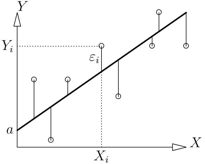
Figure 6.1: Actual observations (points) and plot of the regression (thick line) and residuals (thin lines).

Estimating coefficients

Figure 6.1 shows the observations and the plot of predicted values. The best fit is that which minimizes the residual error. There are several ways of quantifying this residual error. From a mathematical standpoint, this is equivalent with choosing a norm to measure \(\varepsilon\) and various norms could be used. The norm that is commonly used is the \(L_2\) norm, which is equivalent with quantifying the residual difference between the actual observations and the predictions by summing the squares of the residuals, which is also called the sum of squares (SS): \[ \mathrm{SSE}(a,b)=\sum_{i=1}^n\varepsilon_i^2=\sum_{i=1}^n(Y_i-\hat{Y}_i)^2 =\sum_{i=1}^n(Y_i-a-bX_i)^2 \] The best fit is therefore that which minimizes SS. In other words, the estimations \(\hat{a}\) and \(\hat{b}\) of the coefficients \(a\) and \(b\) are values of \(a\) and \(b\) that minimize the sum of squares: \[ (\hat{a},\ \hat{b})=\arg\min_{(a,\ b)}\mathrm{SSE}(a,b) \] This minimum may be obtained by calculating the partial derivatives of SS in relation to \(a\) and \(b\), and by looking for the values of \(a\) and \(b\) that cancel these partial derivatives. Simple calculations yield the following results: \(\hat{b}=\widehat{\mathrm{Cov}}(X,\ Y)/S_X^2\) and \(\hat{a}=\bar{Y}-\hat{b}\bar{X}\), where \(\bar{X}=(\sum_{i=1}^nX_i)/n\) is the empirical mean of the effect variable, \(\bar{Y}=(\sum_{i=1}^nY_i)/n\) is the empirical mean of the response variable, \[ S_X^2=\frac{1}{n}\sum_{i=1}^n(X_i-\bar{X})^2 \] is the empirical variance of the effect variable, and \[ \widehat{\mathrm{Cov}}(X,\ Y)=\frac{1}{n}\sum_{i=1}^n(X_i-\bar{X})(Y_i-\bar{Y}) \] is the empirical covariance between the effect variable and the response variable. The estimation of the residual variance is: \[ \hat{\sigma}^2=\frac{1}{n-2}\sum_{i=1}^n(Y_i-\hat{a}-\hat{b}X_i)^2 =\frac{\mathrm{SSE}(\hat{a},\ \hat{b})}{n-2} \] Because this method of estimating the coefficients is based on minimizing the sum of squares, it is called the least squares method (sometimes it is called the “ordinary least squares” method to differentiate it from the weighted least squares method we will see in § 6.1.3). This estimation method has the advantage of providing an explicit expression of the estimated coefficients.

Interpreting the results of a regression

When fitting a simple linear regression, several outputs need to be analyzed. The determination coefficient, more commonly called \(R^2\), measures the quality of the fit. \(R^2\) is directly related to the residual variance since: \[ R^2=1-\frac{\hat{\sigma}^2(n-2)/n}{S_Y^2} \] where \(S_Y^2=[\sum_{i=1}^n(Y_i-\bar{Y})^2]/n\) is the empirical variance of \(Y\). The difference \(S_Y^2-\hat{\sigma}^2(n-2)/n\) between the variance of \(Y\) and the residual variance corresponds to the variance explained by the model. The determination coefficient \(R^2\) can be interpreted as being the ratio between the variance explained by the model and the total variance. It is between 0 and 1, and the closer it is to 1, the better the quality of the fit. In the case of a simple linear regression, and only in this case, \(R^2\) is also the square of the linear correlation coefficient (also called Pearson’s coefficient) between \(X\) and \(Y\). We have already seen in chapter 5 (particularly in Figure 5.2) that the interpretation of \(R^2\) has its limitations.

In addition to estimating values for coefficients \(a\) and \(b\), model fitting also provides the standard deviations of these estimations (i.e. the standard deviations of estimators \(\hat{a}\) and \(\hat{b}\)), and the results of significance tests on these coefficients. A test is performed on the y-intercept \(a\), which tests the null hypothesis that \(a=0\), and likewise a test is performed on the slope \(b\), which tests the hypothesis that \(b=0\).

Finally, the result given by the overall significance test for the model is also analyzed. This test is based on breaking down the total variance of \(Y\) into the sum of the variance explained by the model and the residual variance. Like in an analysis of variance, the test used is Fisher’s test which, as test statistic, uses a weighted ratio of the explained variance over the residual variance. In the case of a simple linear regression, and only in this case, the test for the overall significance of the model gives the same result as the test on the null hypothesis \(b=0\). This can be grasped intuitively: a line linking \(X\) to \(Y\) is significant only if its slope is not zero.

Checking hypotheses

Model fitting may be brought to a conclusion by checking that the hypotheses put forward for the residuals are in fact satisfied. We will not consider here the hypothesis that the residuals are independent for this has already been satisfied thanks to the sampling plan adopted. If there is a natural order in the observations, we could possibly use the Durbin-Watson test to test if the residuals are indeed independent (Durbin and Watson 1971). The hypothesis that the residuals are normally distributed can be checked visually by inspecting the quantile–quantile graph. This graph plots the empirical quantiles of the residuals against the theoretical quantiles of the standard normal distribution. If the hypothesis that the residuals are normally distributed is satisfied, then the points are approximately aligned along a straight line, as in Figure 6.2 (right plot).

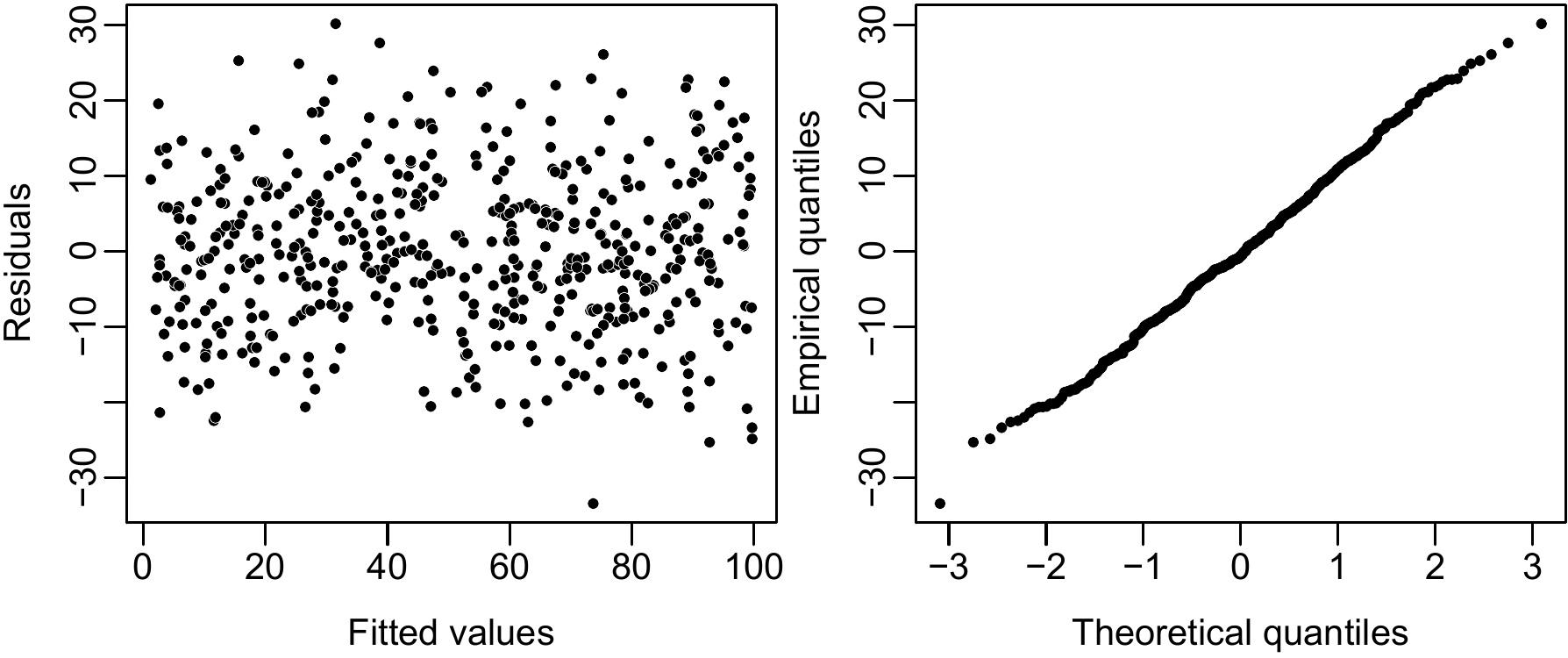
Figure 6.2: Residuals plotted against fitted values (left) and quantile–quantile plot (right) when the normal distribution and constant variance of the residuals hypotheses are satisfied.

In the case of fitting volume or biomass models, the most important hypothesis to satisfy is that of the constant variance of the residuals. This can be checked visually by plotting the cluster of points for the residuals \(\varepsilon_i=Y_i-\hat{Y}_i\) in function to predicted values \(\hat{Y}_i=\hat{a}+\hat{b}X_i\).

If the variance of the residuals is indeed constant, this cluster of points should not show any particular trend and no particular structure. This for instance is the case for the plot shown on the left in Figure 6.2. By contrast, if the cluster of points shows some form of structure, the hypothesis should be questioned. This for instance is the case in Figure 6.3 where the cluster of points for the residuals plotted against fitted values forms a funnel shape. This shape is typical of a residual variance that increases with the effect variable (which we call heteroscedasticity). If this is the case, a model other than a simple linear regression must be fitted.

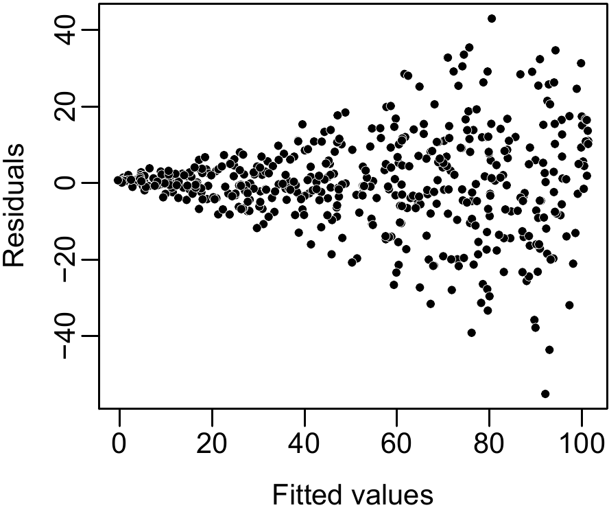
Figure 6.3: Plot of residuals against fitted values when the residuals have a non constant variance (heteroscedasticity).

In the case of biological data such as tree volume or biomass, heteroscedasticity is the rule and homoscedasticity the exception. This means simply that the greater tree biomass (or volume), the greater the variability of this biomass (or volume). This increase in the variability of biomass with increasing size is a general principle in biology. Thus, when fitting biomass or volume models, simple linear regression using biomass as response variable (\(Y=B\)) is generally of little use. The log transformation (i.e. \(Y=\ln(B)\)) resolves this problem and therefore the linear regressions we use for adjusting models nearly always use log-transformed data. We will return at length to this fundamental point later.

Red line 6.1 \(\looparrowright\) Simple linear regression between \(\ln(B)\) and \(\ln(D)\)

The exploratory analysis (red line 5.4) showed that the relation between the log of the biomass and the log of the dbh was linear, with a variance of \(\ln(B)\) that was approximately constant. A simple linear regression may therefore be fitted to predict \(\ln(B)\)from \(\ln(D)\): \[ \ln(B)=a+b\ln(D)+\varepsilon \] where \[ \mathrm{Var}(\varepsilon)=\sigma^2 \] The regression is fitted using the ordinary least squares method. Given that we cannot apply the log transformation to a value of zero, zero biomass data (see red line 4.1) must first be withdrawn from the dataset:

m <- lm(log(Btot) ~ I(log(dbh)), data = dat[dat$Btot > 0,])
summary(m)

The residual standard deviation is \(\hat{\sigma}=0.462\), \(R^2\) is 0.9642 and the model is highly significant (Fisher’s test: \(F_{1,39}=1051\), p-value \(<2.2\times10^{-16}\)). The values of the coefficients are given in the table below:

##             Estimate Std. Error t value Pr(>|t|)    
## (Intercept) -8.42722    0.27915  -30.19   <2e-16 ***
## I(log(dbh))  2.36104    0.07283   32.42   <2e-16 ***

The first column in the table gives the values of the coefficients. The model is therefore: \(\ln(B)=-8.42722+2.36104\ln(D)\). The second column gives the standard deviations of the coefficient estimators. The third column gives the result of the test on the null hypothesis that the coefficient is zero. Finally, the fourth column gives the p-value of this test. In the present case, both the slope and the y-intercept are significantly different from zero. We must now check graphically that the hypotheses of the linear regression are satisfied:

plot(m, which = 1:2)

The result is shown in Figure 6.4. Even though the quantile–quantile plot of the residuals appears to have a slight structure, we will consider that the hypotheses of the simple linear regression are suitably satisfied.

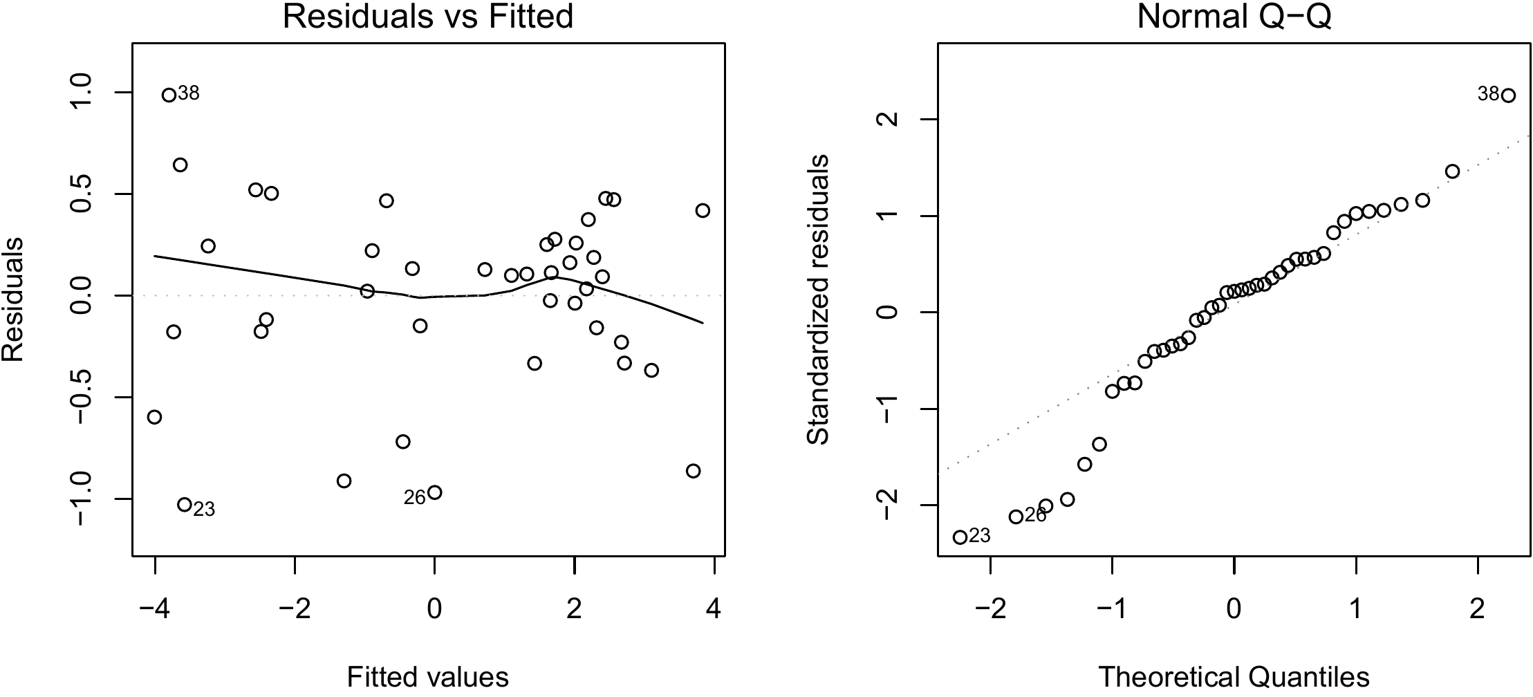
Figure 6.4: Residuals plotted against fitted values (left) and quantile–quantile plot (right) of the residuals of the simple linear regression of \(\ln(B)\) against \(\ln(D)\) fitted for the 42 trees measured by Henry et al. (2010) in Ghana.

Red line 6.2 \(\looparrowright\) Simple linear regression between \(\ln(B)\) and \(\ln(D^2H)\)

The exploratory analysis (red line 5.5) showed that the relation between the log of the biomass and the log of \(D^2H\) was linear, with a variance of \(\ln(B)\) that was approximately constant. We can therefore fit a simple linear regression to predict \(\ln(B)\) from \(\ln(D^2H)\): \[ \ln(B)=a+b\ln(D^2H)+\varepsilon \] where \[ \mathrm{Var}(\varepsilon)=\sigma^2 \] The regression is fitted by the ordinary least squares method. Given that we cannot apply the log transformation to a value of zero, zero biomass data (see red line 4.1) must first be withdrawn from the dataset:

m <- lm(log(Btot) ~ I(log(dbh^2 * heig)), data = dat[dat$Btot > 0,])
summary(m)

The residual standard deviation is \(\hat{\sigma}=0.4084\), \(R^2\) is 0.972 and the model is highly significant (Fisher’s test: \(F_{1,39}=1356\), p-value \(<2.2\times10^{-16}\)). The values of the coefficients are as follows:

##                      Estimate Std. Error t value Pr(>|t|)    
## (Intercept)          -8.99427    0.26078  -34.49   <2e-16 ***
## I(log(dbh^2 * heig))  0.87238    0.02369   36.82   <2e-16 ***

The first column in the table gives the values of the coefficients. The model is therefore: \(\ln(B)=-8.99427+0.87238\ln(D^2H)\). The second column gives the standard deviations of the coefficient estimators. The third column gives the result of the test on the null hypothesis that “the coefficient is zero”. Finally, the fourth column gives the p-value of this test. In the present case, both the slope and the y-intercept are significantly different from zero.

We must now check graphically that the hypotheses of the linear regression are satisfied:

plot(m, which = 1:2)

The result is shown in Figure 6.5. Even though the plot of the residuals against the fitted values appears to have a slight structure, we will consider that the hypotheses of the simple linear regression are suitably satisfied.

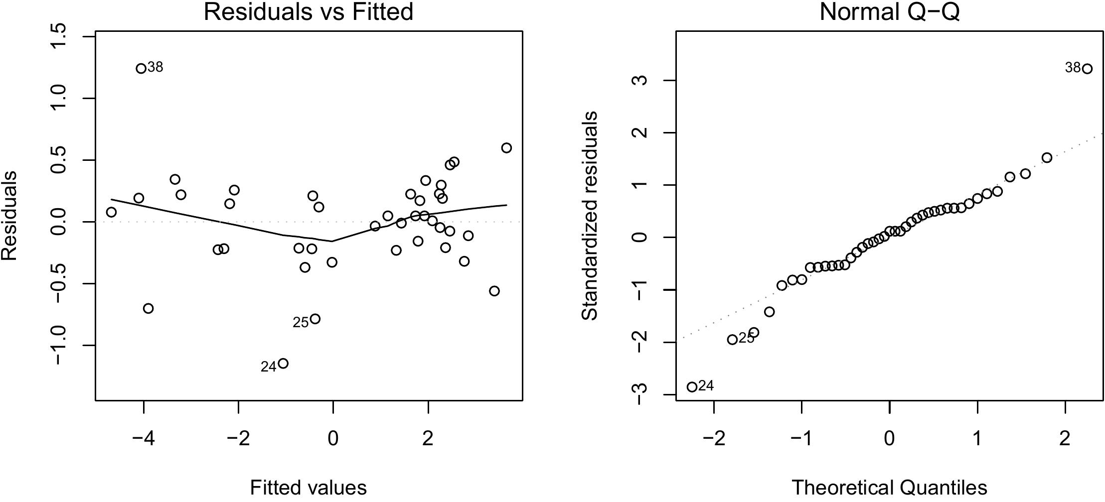
Figure 6.5: Residuals plotted against fitted values (left) and quantile–quantile plot (right) of the residuals of the simple linear regression of \(\ln(B)\) against \(\ln(D^2H)\) fitted for the 42 trees measured by Henry et al. (2010) in Ghana.

6.1.2 Multiple regression

Multiple regression is the extension of simple linear regression to the case where there are several effect variables, and is written: \[\begin{equation} Y=a_0+a_1X_1+a_2X_2+\ldots+a_pX_p+\varepsilon\tag{6.3} \end{equation}\] where \(Y\) is the response variable, \(X_1\), \(\ldots\), \(X_p\) the \(p\) effect variables, \(a_0\), \(\ldots\), \(a_p\) the coefficients to be estimated, and \(\varepsilon\) the residual error. Counting the y-intercept \(a_0\), there are \(p+1\) coefficients to be estimated. Like for simple linear regression, the variance of the residuals is assumed to be constant and equal to \(\sigma^2\): \[ \varepsilon\;\mathop{\sim}_{\mathrm{i.i.d.}}\;\mathcal{N}(0,\ \sigma) \] The following biomass models are examples of multiple regressions: \[\begin{eqnarray} \ln(B) &=& a_0+a_1\ln(D^2H)+a_2\ln(\rho)+\varepsilon\tag{6.4}\\ % \ln(B) &=& a_0+a_1\ln(D)+a_2\ln(H)+\varepsilon\tag{6.5}\\ % \ln(B) &=& a_0+a_1\ln(D)+a_2\ln(H)+a_3\ln(\rho)+\varepsilon\tag{6.6}\\ % \ln(B) &=& a_0+a_1\ln(D)+a_2[\ln(D)]^2+a_3[\ln(D)]^3+\varepsilon\tag{6.7}\\ % \ln(B) &=& a_0+a_1\ln(D)+a_2[\ln(D)]^2+a_3[\ln(D)]^3+a_4\ln(\rho)+\varepsilon\tag{6.8}% \end{eqnarray}\] where \(\rho\) is wood density. In all these examples the response variable is the log of the biomass: \(Y=\ln(B)\). As model (6.4) generalizes (6.2) by adding dependency on wood specific density: typically (6.4) should be preferred to (6.2) when the dataset is multispecific. Model (6.5) generalizes (6.2) by considering that the exponent associated with height \(H\) is not necessarily half the exponent associated with dbh. It therefore introduces a little more flexibility into the form of the relation between biomass and \(D^2H\). Model (6.6) generalizes (6.2) by considering that there are both several species and that biomass is not quite a power of \(D^2H\). Model (6.7) generalizes (6.1) by considering that the relation between \(\ln(B)\) and \(\ln(D)\) is not exactly linear. It therefore offers a little more flexibility in the form of this relation. Model (6.8) is the extension of (6.7) to take account of the presence of several species in a dataset.

Estimating coefficients

In the same manner as for simple linear regression, the estimation of the coefficients is based on the least squares method. Estimators \(\hat{a}_0\), \(\hat{a}_1\), \(\ldots\), \(\hat{a}_p\) are the values of coefficients \(a_0\), \(a_1\), \(\ldots\), \(a_p\) that minimize the sum of squares: \[ \mathrm{SSE}(a_0,\ a_1,\ \ldots,\ a_p)=\sum_{i=1}^n\varepsilon_i^2 =\sum_{i=1}^n(Y_i-\hat{Y}_i)^2 =\sum_{i=1}^n(Y_i-a_0-a_1X_{i1}-\ldots-a_pX_{ip})^2 \] where \(X_{ij}\) is the value of the \(j\)th effect variable for the \(i\)th observation (\(i=1\), \(\ldots\), \(n\) and \(j=1\)  \(\ldots\), \(p\)). Once again, estimations of the coefficients may be obtained by calculating the partial derivatives of SS in relation to the coefficients, and by looking for the values of the coefficients that cancel these partial derivatives. These computations are barely more complex than for simple linear regression, on condition that they are arranged in a matrix form. Let \(\mathbf{X}\) be the matrix with \(n\) lines and \(p\) columns, called the design matrix, containing the values observed for the effect variables: \[ \mathbf{X}=\left[ \begin{array}{cccc} 1 & X_{11} & \cdots & X_{1p}\\ % \vdots & \vdots & & \vdots\\ % 1 & X_{n1} & \cdots & X_{np}\\ % \end{array} \right] \] Let \(\mathbf{Y}={}^{\mathrm{t}}{[Y_1,\ \ldots,\ Y_n]}\) be the vector of the \(n\) values observed for the response variable, and \(\mathbf{a}={}^{\mathrm{t}}{[a_0,\ \ldots,\ a_p]}\) be the vector of the \(p+1\) coefficients to be estimated. Thus \[ \mathbf{X}\mathbf{a}=\left[ \begin{array}{c} a_0+a_1X_{11}+\ldots+a_pX_{1p}\\ % \vdots\\ % a_0+a_1X_{n1}+\ldots+a_pX_{np}\\ % \end{array} \right] \] is none other than the vector \(\hat{\mathbf{Y}}\) of the \(n\) values fitted by the response variable model. Using these matrix notations, the sum of squares is written: \[ \mathrm{SSE}(\mathbf{a})={}^{\mathrm{t}}{(\mathbf{Y}-\hat{\mathbf{Y}})} (\mathbf{Y}-\hat{\mathbf{Y}})={}^{\mathrm{t}}{(\mathbf{Y}-\mathbf{X}\mathbf{a})} (\mathbf{Y}-\mathbf{X}\mathbf{a}) \] And using matrix differential calculus (Magnus and Neudecker 2007), we finally obtain: \[ \hat{\mathbf{a}}=\arg\min_{\mathbf{a}}\mathrm{SSE}(\mathbf{a}) =({}^{\mathrm{t}}{\mathbf{X}}\mathbf{X})^{-1}{}^{\mathrm{t}}{\mathbf{X}}\mathbf{Y} \] The estimation of the residual variance is: \[ \hat{\sigma}^2=\frac{\mathrm{SSE}(\hat{\mathbf{a}})}{n-p-1} \] Like for simple linear regression, this estimation method has the advantage of providing an explicit expression of the coefficients estimated. As simple linear regression is a special case of multiple regression (case where \(p=1\)), we can check that the matrix expressions for estimating the coefficients and \(\hat{\sigma}\) actually — when \(p=1\) — give again the expressions given previously with a simple linear regression.

Interpreting the results of a multiple regression

In the same manner as for simple linear regression, fitting a multiple regression provides a determination coefficient \(R^2\) corresponding to the proportion of the variance explained by the model, values \(\hat{\mathbf{a}}\) for model coefficients \(a_0\), \(a_1\), \(\ldots\), \(a_p\), standard deviations for these estimations, the results of significance tests on these coefficients (there are \(p+1\) — one for each coefficient — null hypotheses \(a_i=0\) for \(i=0\), \(\ldots\), \(p\)), and the result of the test on the overall significance of the model.

As previously, \(R^2\) has a value of between 0 and 1. The higher the value, the better the fit. However, it should be remembered that the value of \(R^2\) increases automatically with the number of effect variables used. For instance, if we are predicting \(Y\) using a polynomial with \(p\) orders in \(X\), \[ Y=a_0+a_1X+a_2X^2+\ldots+a_pX^p \] \(R^2\) will automatically increase with the number of orders \(p\). This may give the illusion that the higher the number of orders \(p\) in a polynomial, the better its fit. This of course is not the case. If the number \(p\) of orders is too high, this will result in model over-parameterization. In other words, \(R^2\) is not a valid criterion on which model selection may be based. We will return to this point in section 6.3.

Checking hypotheses

Like simple linear regression, multiple regression is based on three hypotheses: that the residuals are independent, that they follow a normal distribution and that their variance is constant. These hypotheses may be checked in exactly the same manner as for the simple linear regression. To check that the residuals follow a normal distribution, we can plot a quantile–quantile graph and verify visually that the cluster of points forms a straight line. To check that the variance of the residuals is constant, we can plot the residuals against the fitted values and verify visually that the cluster of points does not show any particular trend. The same restriction as for the simple linear regression applies to volume or biomass data that nearly always (or always) show heteroscedasticity. For this reason, multiple regression is generally applicable for fitting models only on log-transformed data.

Red line 6.3 \(\looparrowright\) Polynomial regression between \(\ln(B)\) and \(\ln(D)\)

The exploratory analysis (red line 5.4) showed that the relation between the log of the biomass and the log of the dbh was linear. We can ask ourselves the question of whether this relation is truly linear, or has a more complex shape. To do this, we must construct a polynomial regression with \(p\) orders, i.e. a multiple regression of \(\ln(B)\) against \(\ln(D)\), \([\ln(D)]^2\), \(\ldots\), \([\ln(D)]^p\): \[ \ln(B)=a_0+a_1\ln(D)+a_2[\ln(D)]^2+\ldots+a_p[\ln(D)]^p+\varepsilon \] where \[ \mathrm{Var}(\varepsilon)=\sigma^2 \] The regression is fitted by the ordinary least squares method. As the log transformation stabilizes the residual variance, the hypotheses on which the multiple regression is based are in principle satisfied. For a second-order polynomial, the polynomial regression is fitted by the following code:

m2 <- lm(log(Btot) ~ I(log(dbh)) + I(log(dbh)^2), data = dat[dat$Btot > 0,])
print(summary(m2))

This yields:

##                Estimate Std. Error t value Pr(>|t|)    
## (Intercept)   -8.322190   1.031359  -8.069 9.25e-10 ***
## I(log(dbh))    2.294456   0.633072   3.624 0.000846 ***
## I(log(dbh)^2)  0.009631   0.090954   0.106 0.916225

with \(R^2=\) 0.9642. And as for a third-order polynomial regression:

m3 <- lm(
  log(Btot) ~ I(log(dbh)) + I(log(dbh)^2) + I(log(dbh)^3),
  data = dat[dat$Btot > 0,]
  )
print(summary(m3))

it yields:

##               Estimate Std. Error t value Pr(>|t|)
## (Intercept)   -5.46413    3.80855  -1.435    0.160
## I(log(dbh))   -0.42448    3.54394  -0.120    0.905
## I(log(dbh)^2)  0.82073    1.04404   0.786    0.437
## I(log(dbh)^3) -0.07693    0.09865  -0.780    0.440

with \(R^2=\) 0.9648. Finally, a fourth-order polynomial regression:

m4 <- lm(
  log(Btot) ~ I(log(dbh)) + I(log(dbh)^2) + I(log(dbh)^3) + I(log(dbh)^4),
  data = dat[dat$Btot > 0,]
  )
print(summary(m4))

yields:

##               Estimate Std. Error t value Pr(>|t|)  
## (Intercept)   -26.7953    15.7399  -1.702   0.0973 .
## I(log(dbh))    26.3990    19.5353   1.351   0.1850  
## I(log(dbh)^2) -11.2782     8.7301  -1.292   0.2046  
## I(log(dbh)^3)   2.2543     1.6732   1.347   0.1863  
## I(log(dbh)^4)  -0.1628     0.1166  -1.396   0.1714

with \(R^2=\) 0.9648. Adding higher order terms above 1 therefore does not improve the model. The coefficients associated with these terms were not significantly different from zero. But the model’s \(R^2\) continued to increase with the number \(p\) of orders in the polynomial. \(R^2\) is not therefore a reliable criterion for selecting the order of the polynomial. The plots fitted by these different polynomials may be superimposed on the biomass-dbh cluster of points: with object m indicating the linear regression of \(\ln(B)\) against \(\ln(D)\) fitted in red line 6.1,

m <- lm(log(Btot) ~ I(log(dbh)), data = dat[dat$Btot > 0,]) ## Red line 7

with(dat, plot(
  x = dbh, y = Btot, xlab = "Dbh (cm)", ylab = "Biomass (t)", log = "xy"
  ))
D <- 10^seq(par("usr")[1], par("usr")[2], length = 200)
lines(D, exp(predict(m , newdata = data.frame(dbh = D))))
lines(D, exp(predict(m2, newdata = data.frame(dbh = D))))
lines(D, exp(predict(m3, newdata = data.frame(dbh = D))))
lines(D, exp(predict(m4, newdata = data.frame(dbh = D))))

The plots are shown in Figure 6.6: the higher the order of the polynomial, the more deformed the plot in order to fit the data, with increasingly unrealistic extrapolations outside the range of the data (typical of model over-parameterization).

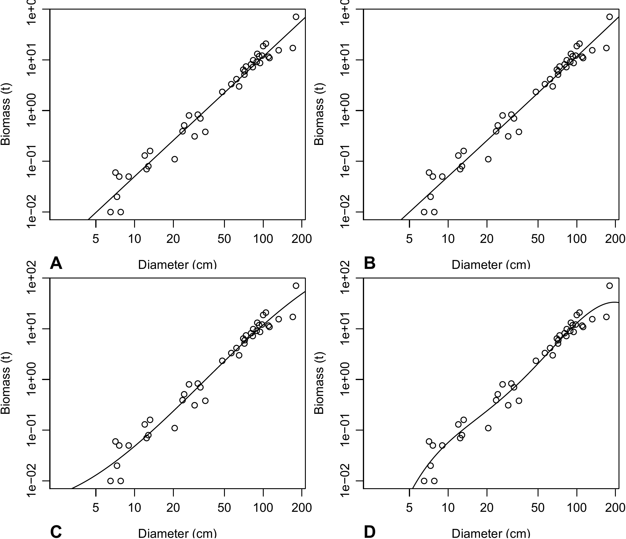
Figure 6.6: Biomass against dbh for 42 trees in Ghana measured by Henry et al. (2010) (points), and predictions (plots) by a polynomial regression of \(\ln(B)\) against \(\ln(D)\): (A) first-order polynomial (straight line); (B) second-order polynomial (parabolic); (C) third-order polynomial; (D) fourth-order polynomial.

Red line 6.4 \(\looparrowright\) Multiple regression between \(\ln(B)\), \(\ln(D)\) and \(\ln(H)\)

The graphical exploration (red lines 5.2 and 5.5) showed that the combined variable \(D^2H\) was linked to biomass by a power relation (i.e. a linear relation on a log scale): \(B=a(D^2H)^b\). We can, however, wonder whether the variables \(D^2\) and \(H\) have the same exponent \(b\), or whether they have different exponents: \(B=a\times(D^2)^{b_1}H^{b_2}\). Working on the log-transformed data (which in passing stabilizes the residual variance), means fitting a multiple regression of \(\ln(B)\) against \(\ln(D)\) and \(\ln(H)\): \[ \ln(B)=a+b_1\ln(D)+b_2\ln(H)+\varepsilon \] where \[ \mathrm{Var}(\varepsilon)=\sigma^2 \] The regression is fitted by the ordinary least squares method. Fitting this multiple regression:

m <- lm(log(Btot) ~ I(log(dbh)) + I(log(heig)), data = dat[dat$Btot > 0,])
summary(m)

yields:

##              Estimate Std. Error t value Pr(>|t|)    
## (Intercept)   -8.9050     0.2855 -31.190  < 2e-16 ***
## I(log(dbh))    1.8654     0.1604  11.632 4.35e-14 ***
## I(log(heig))   0.7083     0.2097   3.378   0.0017 **

with a residual standard deviation of 0.4104 and \(R^2=\) 0.9725 (0.971). The model is highly significant (Fisher’s test: \(F_{2,38}=671.5\), p-value \(<2.2\times10^{-16}\)). The model, all of whose coefficients are significantly different from zero, is written: \(\ln(B)=-8.9050+1.8654\ln(D)+0.7083\ln(H)\). By applying the exponential function to return to the starting data, the model becomes: \(B=1.357\times10^{-4}D^{1.8654}H^{0.7083}\). The exponent associated with height is a little less than half that associated with dbh, and is a little less than the exponent of 0.87238 found for the combined variable \(D^2H\) (see red line 6.2). An examination of the residuals:

plot(m, which = 1:2)

shows nothing in particular (Figure 6.7).

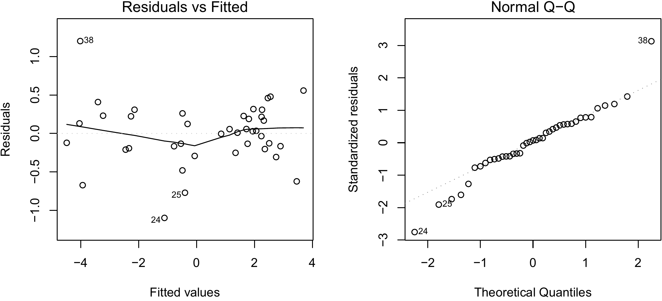
Figure 6.7: Residuals plotted against fitted values (left) and quantile–quantile plot (right) for residuals of the multiple regression of \(\ln(B)\) against \(\ln(D)\) and \(\ln(H)\) fitted for the 42 trees measured by Henry et al. (2010) in Ghana.

6.1.3 Weighted regression

Let us now suppose that we want to fit directly a polynomial model of biomass \(B\) against \(D\). For example, for a second-order polynomial: \[\begin{equation} B=a_0+a_1D+a_2D^2+\varepsilon\tag{6.9} \end{equation}\] As mentioned earlier, the variability of the biomass nearly always (if not always\(\ldots\)) increases with tree dbh \(D\). In other words, the variance of \(\varepsilon\) increases with \(D\), in contradiction with the homoscedasticity hypothesis required by multiple regression. Therefore, model (6.9) cannot be fitted by multiple regression. Log transformation stabilizes the residual variance (we will return to this in section 6.1.5). If we take \(\ln(B)\) as the response variable, the model becomes: \[\begin{equation} \ln(B)=\ln(a_0+a_1D+a_2D^2)+\varepsilon\tag{6.10} \end{equation}\] It is reasonable to assume that the variance of the residuals in such a model is constant. But unfortunately, this is no longer a linear model as the dependency of the response variables on the coefficients \(a_0\), \(a_1\) and \(a_2\) is not linear. Therefore, model (6.10) cannot be fitted by a linear model. We will see later (§ 6.2) how to fit this non-linear model.

A weighted regression can be used to fit a model such as (6.9) where the variance of the residuals is not constant, while nevertheless using the formalism of the linear model. It may be regarded as extending multiple regression to the case where the variance of the residuals is not constant. Weighted regression was developed in forestry between the 1960s and the 1980s, particularly thanks to the work of Cunia (1964); Cunia (1987c). It was widely used to fit linear tables (Whraton and Cunia 1987; Brown, Gillespie, and Lugo 1989; Parresol 1999), before being replaced by more efficient fitting methods we will see in section 6.1.4.

A weighted regression is written in an identical fashion to the multiple regression (6.3): \[ Y=a_0+a_1X_1+a_2X_2+\ldots+a_pX_p+\varepsilon \] except that it is no longer assumed that the variance of the residuals is constant. Each observation now has its own residual variance \(\sigma_i^2\): \[ \varepsilon_i\sim\mathcal{N}(0,\ \sigma_i) \] Each observation is associated with a positive weight \(w_i\) (hence the term “weighted” to describe this regression), which is inversely proportional to the residual variance: \[ w_i\propto1/\sigma_i^2 \] The proportionality coefficient between \(w_i\) and \(1/\sigma_i^2\) does not need to be specified as the method is insensitive to any renormalization of the weights (as we shall see in the next section). Associating each observation with a weight inversely proportional to its variance is quite natural. If an observation has a very high residual variance, this means that it has very high intrinsic variability, and it is therefore quite natural that it has less weight in model fitting. As we cannot estimate \(n\) weights from \(n\) observations, we must model the weighting. When dealing with biological data such as biomass or volume, heteroscedasticity of the residuals corresponds nearly always to a power relation between the residual variance and the size of the trees. We may therefore assume that among the \(p\) effect variables of the weighted regression, there is one (typically tree dbh) such that \(\sigma_i\) is a power relation of this variable. Without loss of generality, we can put forward that this variable is \(X_1\), such that: \[ \sigma_i=k\ X_{i1}^c \] where \(k>0\) and \(c\geq0\). In consequence: \[ w_i\propto X_{i1}^{-2c} \] The exponent \(c\) cannot be estimated in the same manner as \(a_0\), \(a_1\), \(\ldots\), \(a_p\), but must be fixed in advance. This is the main drawback of this fitting method. We will see later how to select a value for exponent \(c\). By contrast, the multiplier \(k\) does not need to be estimated as the weights \(w_i\) are defined only to within a multiplier factor. In practice therefore we can put forward \(w_i=X_{i1}^{-2c}\).

Estimating coefficients

The least squares method is adjusted to take account of the weighting of the observations. We therefore speak of the weighted least squares method. For a fixed exponent \(c\), estimations of coefficients \(a_0\), \(\ldots\), \(a_p\) have values that minimize the weighted sum of squares: \[ \mathrm{SSE}(a_0,\ a_1,\ \ldots,\ a_p)=\sum_{i=1}^nw_i\ \varepsilon_i^2 =\sum_{i=1}^nw_i(Y_i-a_0-a_1X_{i1}-\ldots-a_pX_{ip})^2 \] or as a matrix: \[ \mathrm{SSE}(\mathbf{a})={}^{\mathrm{t}}{(\mathbf{Y}-\hat{\mathbf{Y}})}\mathbf{W} (\mathbf{Y}-\hat{\mathbf{Y}})={}^{\mathrm{t}}{(\mathbf{Y}-\mathbf{X}\mathbf{a})} \mathbf{W} (\mathbf{Y}-\mathbf{X}\mathbf{a}) \] where \(\mathbf{W}\) is the \(n\times n\) diagonal matrix with \(w_i\) on its diagonal: \[ \mathbf{W}=\left[ \begin{array}{ccc} w_1 && \mathbf{0}\\ % & \ddots & \\ % \mathbf{0} && w_n \end{array} \right] \] The least SS is obtained for (Magnus and Neudecker 2007): \[ \hat{\mathbf{a}}=\arg\min_{\mathbf{a}}\mathrm{SSE}(\mathbf{a}) =({}^{\mathrm{t}}{\mathbf{X}}\mathbf{W}\mathbf{X})^{-1}{}^{\mathrm{t}}{\mathbf{X}}\mathbf{W}\mathbf{Y} \] This minimum does not change when all the weights \(w_i\) are multiplied by the same scalar, clearly proving that the method is not sensitive to normalization of weights. We can check that the estimation yielded by the weighted least squares method applied to observations \(X_{ij}\) and \(Y_i\) gives the same result as that yielded by the ordinary least squares method applied to observations \(\sqrt{w_i}\ X_{ij}\) and \(\sqrt{w_i}\ Y_i\). Like previously, this fitting method has the advantage that the estimations of the coefficients have an explicit expression.

Interpreting results and checking hypotheses

The results of the weighted regression are interpreted in exactly the same fashion as for the multiple regression. The same may also be said of the residuals-related hypotheses, except that the residuals are replaced by the weighted residuals \(\varepsilon'_i=\sqrt{w_i}\ \varepsilon_i=\varepsilon_i/X_i^c\). The graph of the weighted residuals \(\varepsilon_i'\) against the fitted values must not show any particular trend (like in Figure 6.8B). If the cluster of points given by plotting the residuals against the fitted values takes on a funnel-like shape open toward the right (as in Figure 6.8A), then the value of exponent \(c\) is too low (the lowest possible value being zero). If the cluster of points takes on a funnel-like shape closed toward the right (as in Figure 6.8C), then the value of exponent \(c\) is too high.

Figure 6.8: Plot of weighted residuals against fitted values for a weighted regression: (A) the value of exponent \(c\) is too low for the weighting; (B) the value of exponent \(c\) is appropriate; (C) the value of exponent \(c\) is too high. It should be noted that as the value of c increases, the rank of the values for the weighted values \(\varepsilon/X^c\) decreases.

Choosing the right weighting

A crucial point in weighted regression is the prior selection of a value for exponent c that defines the weighting. Several methods can be used to determine \(c\). The first consists in proceeding by trial and error based on the appearance of the plot of the residuals against the fitted values. As the appearance of the plot provides information on the pertinence of the value of \(c\) (Figure 6.8), several values of \(c\) can simply be tested until the cluster of points formed by plotting the weighted residuals against the fitted values no longer shows any particular trend.

As linear regression is robust with regard to the hypothesis that the variance of the residuals is constant, there is no need to determine \(c\) with great precision. In most cases it is enough to test integers of \(c\). In practice, the weighted regression may be fitted for \(c\) values of 0, 1, 2, 3 or 4 (it is rarely useful to go above 4), and retain the integer value that yields the best appearance for the cluster of points in the plot of the weighted residuals against the fitted values. This simple method is generally amply sufficient.

If we are looking to obtain a more precise value for exponent \(c\), we can calculate approximately the conditional variance of response variable \(Y\) as we know \(X_1\):

1. divide \(X_1\) into \(K\) classes centered on \(X_{1k}\) (\(k=1\), \(\ldots\), \(K\));
2. calculate the empirical variance, \(\sigma^2_k\), of \(Y\) for the observations in class \(k\) (avec \(k=1\), \(\ldots\), \(K\));
3. plot the linear regression of \(\ln(\sigma_k)\) against \(\ln(X_{1k})\).

The slope of this regression is an estimation of \(c\).

The third way of estimating \(c\) consists in looking for the value of \(c\) that minimizes Furnival (1961) index.

Red line 6.5 \(\looparrowright\) Weighted linear regression between \(B\) and \(D^2H\)

The exploratory analysis of the relation between biomass and \(D^2H\) showed (red line 5.2) that this relation is linear, but that the variance of the biomass increases with \(D^2H\). We can therefore fit a weighted linear regression of biomass \(B\) against \(D^2H\): \[ B=a+bD^2H+\varepsilon \] where \[ \mathrm{Var}(\varepsilon)\propto D^{2c} \] The linear regression is fitted by the weighted least squares method, meaning that we must beforehand know the value of exponent \(c\). Let us first estimate coefficient \(c\) for the weighting of the observations. To do this we must divide the observations into dbh classes and calculate the standard deviation of the biomass in each dbh class:

D <- quantile(dat$dbh, (0:5) / 5)
i <- findInterval(dat$dbh, D, rightmost.closed = TRUE)
sdB <- data.frame(D = (D[-1] + D[-6]) / 2, sdB = tapply(dat$Btot, i, sd))

Object D contains the bounds of the dbh classes that are calculated such to have 5 classes containing approximately the same number of observations: Object i contains the number of the dbh class to which each observation belongs. Figure 6.9, obtained by the command:

with(sdB, plot(
  x = D, 
  y = sdB, 
  log = "xy", 
  xlab = "Diameter (cm)", 
  ylab = "Biomass standard deviation (t)"
  ))

shows a plot of the standard deviation of the biomass against the median dbh of each dbh class, on a log scale. The points are roughly aligned along a straight line, confirming that the power model is appropriate for modeling the residual variance. The linear regression of the log of the standard deviation of the biomass against the log of the median dbh for each class, fitted by the command:

summary(lm(log(sdB) ~ I(log(D)), data = sdB))

yields:

##             Estimate Std. Error t value Pr(>|t|)   
## (Intercept)  -7.3487     0.7567  -9.712  0.00232 **
## I(log(D))     2.0042     0.1981  10.117  0.00206 **

The slope of the regression corresponds to \(c\), and is \(2\). Thus, the standard deviation \(\sigma\) of the biomass is approximately proportional to \(D^2\), and we will select a weighting of the observations that is inversely proportional to \(D^4\). The weighted regression of biomass \(B\) against \(D^2H\) with this weighting, and fitted by the command:

m <- lm(Btot ~ I(dbh^2 * heig), data = dat, weights = 1 / dat$dbh^4)
summary(m)

yields:

##                  Estimate Std. Error t value Pr(>|t|)    
## (Intercept)     1.181e-03  2.288e-03   0.516    0.608    
## I(dbh^2 * heig) 2.742e-05  1.527e-06  17.957   <2e-16 ***

An examination of the result of this fitting shows that the y-intercept is not significantly different from zero. This leads us to fit a new weighted regression of biomass \(B\) against \(D^2H\) without an intercept:

m <- lm(Btot ~ -1 + I(dbh^2 * heig), data = dat, weights = 1 / dat$dbh^4)
summary(m)

which yields:

##                  Estimate Std. Error t value Pr(>|t|)    
## I(dbh^2 * heig) 2.747e-05  1.511e-06   18.19   <2e-16 ***

The model is therefore: \(B=2.747\times10^{-5}D^2H\), with \(R^2\) = 0.8897 and a residual standard deviation \(k=0.0003513\) tonnes cm^-2. The model is highly significant (Fisher’s test: \(F_{1,41}=330.8\), p-value \(<2.2\times10^{-16}\)). As this model was fitted directly on non-transformed data, it should be noted that it was unnecessary to withdraw the observations of zero biomass (unlike the situation in red line 6.2). Figure 6.10A, obtained by the command:

plot(
  x = fitted(m),  
  y = residuals(m) / dat$dbh^2, 
  xlab = "Fitted values", 
  ylab = "Weighted residuals"
  )

gives a plot of the weighted residuals against the fitted values. By way of a comparison, Figure 6.10B shows a plot of the weighted residuals against the fitted values when the weighting is too low (with weights inversely proportional to \(D^2\)):

m <- lm(Btot ~ -1 + I(dbh^2 * heig), data = dat, weights = 1 / dat$dbh^2)
plot(
  x = fitted(m), 
  y = residuals(m) / dat$dbh, 
  xlab = "Fitted values", 
  ylab = "Weighted residuals"
  )

whereas 6.10C shows a plot of the weighted residuals against the fitted values when the weighting is too high (with weights inversely proportional to \(D^5\)):

m <- lm(Btot ~ -1 + I(dbh^2 * heig), data = dat, weights = 1 / dat$dbh^5)
plot(
  x = fitted(m), 
  y = residuals(m) / dat$dbh^2.5, 
  xlab = "Fitted values", 
  ylab = "Weighted residuals"
  )

Thus, the coefficient \(c=2\) for the weighting indeed proves to be that which is suitable.

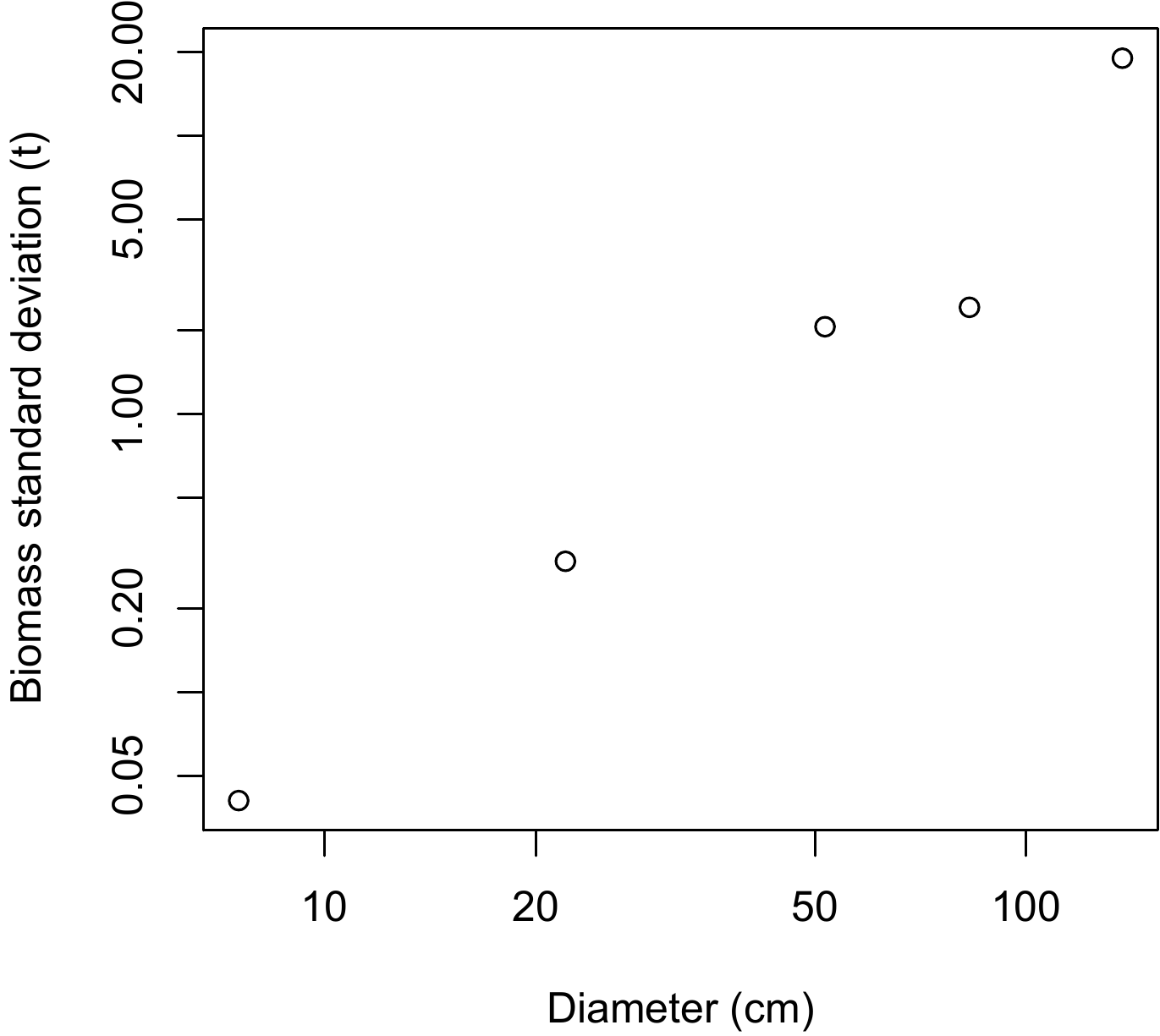
Figure 6.9: Plot of standard deviation of biomass calculated in five dbh classes against median dbh of the class (on a log scale), for 42 trees measured in Ghana by Henry et al. (2010).

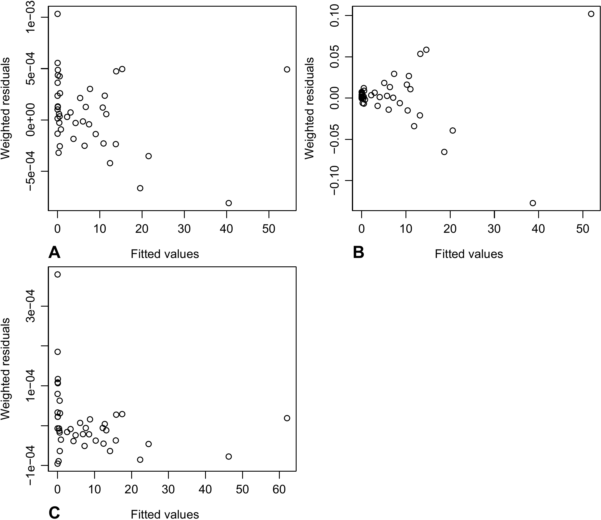
Figure 6.10: Plot of weighted residuals against fitted values for a weighted regression of biomass against \(D^2H\) for 42 trees measured in Ghana by Henry et al. (2010): (A) the weighting is inversely proportional to \(D^4\); (B) the weighting is inversely proportional to \(D^2\); (C) the weighting is inversely proportional to \(D^5\).

Red line 6.6 \(\looparrowright\) Weighted polynomial regression between \(B\) and \(D\)

The exploratory analysis (red line 5.1) showed that the relation between biomass and dbh was parabolic, with the variance of the biomass increasing with dbh. Log-transformation rendered the relation between biomass and dbh linear, but we can also model the relation between biomass and dbh directly by a parabolic relation: \[ B=a_0+a_1D+a_2D^2+\varepsilon \] where \[ \mathrm{Var}(\varepsilon)\propto D^{2c} \] In red line 6.5 we saw that the value \(c=2\) of the exponent was suitable for modeling the conditional standard deviation of the biomass when we know the dbh. We will therefore fit the multiple regression using the weighted least squares method with weighting of the observations proportional to \(1/D^4\):

which yields:

##               Estimate Std. Error t value Pr(>|t|)    
## (Intercept)  1.127e-02  6.356e-03   1.772  0.08415 .  
## dbh         -7.297e-03  2.140e-03  -3.409  0.00153 ** 
## I(dbh^2)     1.215e-03  9.014e-05  13.478 2.93e-16 ***

with a residual standard deviation \(k=\)  tonnes~cm^-2 and \(R^2=\) . The y-intercept is not significantly different from zero. We can therefore again fit a parabolic relation but without the intercept:

m <- lm(Btot ~ -1 + dbh + I(dbh^2), data = dat, weights = 1 / dat$dbh^4)
summary(m)

which yields:

##            Estimate Std. Error t value Pr(>|t|)    
## dbh      -3.840e-03  9.047e-04  -4.245 0.000126 ***
## I(dbh^2)  1.124e-03  7.599e-05  14.789  < 2e-16 ***

with a residual standard deviation \(k=\)  tonnes cm^-2 and \(R^2=\) . The model is highly significant (Fisher’s test: \(F_{2,40}=124.4\), p-value \(< 2.2\times10^{-16}\)) and is written: \(B=-3.840\times10^{-3}D+1.124\times10^{-3}D^2\). Figure 6.11 obtained by the command:

plot(
  x = fitted(m), 
  y = residuals(m) / dat$dbh^2,
  xlab = "fitted values", 
  ylab = "Weighted residuals"
  )

gives a plot of the weighted residuals against the fitted values.

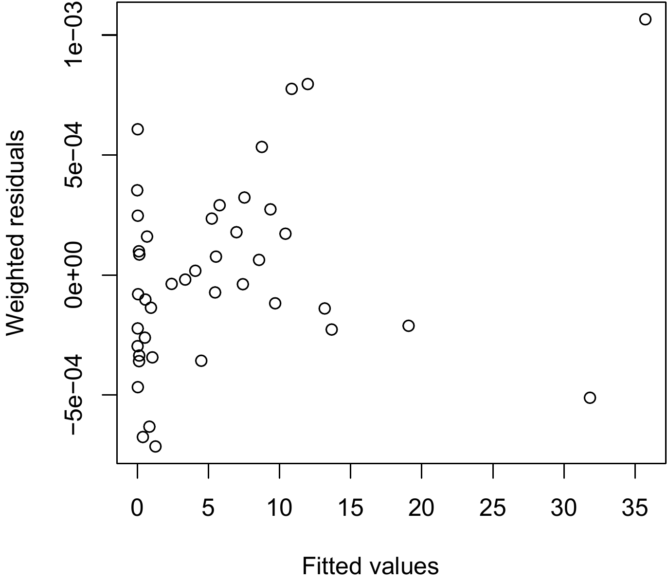
Figure 6.11: Plot of weighted residuals against fitted values for a weighted regression of biomass against \(D\) and \(D^2\) for 42 trees measured in Ghana by Henry et al. (2010).

6.1.4 Linear regression with variance model

An alternative to the weighted regression is to use explicitly a model for the variance of the residuals. As previously, it is realistic to assume that there is an effect variable (without loss of generality, the first) such that the residual standard deviation is a power function of this variable: \[\begin{equation} \mathrm{Var}(\varepsilon)=(kX_1^c)^2\tag{6.11} \end{equation}\] where \(k>0\) and \(c\geq0\). The model is therefore written: \[\begin{equation} Y=a_0+a_1X_1+a_2X_2+\ldots+a_pX_p+\varepsilon\tag{6.12} \end{equation}\] where: \[ \varepsilon\sim\mathcal{N}(0,\ kX_1^c) \] In its form the model is little different from the weighted regression. Regarding its content, it has one fundamental difference: the coefficients \(k\) and \(c\) are now model parameters that need to be estimated, in the same manner as coefficients \(a_0\), \(a_1\), \(\ldots\), \(a_p\). Because of these \(k\) and \(c\) parameters that need to be estimated, the least squares method can no longer be used to estimate model coefficients. Another estimation method has to be used, the maximum likelihood method. Strictly speaking, the model defined by (6.11) and (6.12) is not a linear model. It is far closer conceptually to the non-linear model we will see in section 6.2. We will not go any further here in presenting the non-linear model: the model fitting method defined by (6.11) and (6.12) will be presented as a special case of the non-linear model in section 6.2.

Red line 6.7 \(\looparrowright\) Polynomial regression between \(B\) and \(D\) with variance model

Pre-empting section 6.2, we will fit a linear regression of biomass against \(D^2H\) by specifying a power model on the residual variance: \[ B=a+bD^2H+\varepsilon \] where \[ \mathrm{Var}(\varepsilon)=(kD^c)^2 \] We will see later (§ 6.2) that this model is fitted by maximum likelihood. This regression is in spirit very similar to the previously-constructed weighted regression of biomass against \(D^2H\) (red line 6.5), except that exponent \(c\) used to define the weighting of the observations is now a parameter that must be estimated in its own right rather than a coefficient that is fixed in advance. The linear regression with variance model is fitted as follows:

library(nlme)
start <- coef(lm(Btot ~ I(dbh^2 * heig), data = dat))
names(start) <- c("a", "b")
summary(nlme(
  model   = Btot ~ a + b * dbh^2 * heig, 
  data    = cbind(dat, g = "a"), 
  fixed   = a + b ~ 1, 
  start   = start, 
  groups  = ~g, 
  weights = varPower(form=~dbh)
  ))

and yields (we will return in section 6.2 to the meaning of the start object start):

##          Value    Std.Error DF    t-value      p-value
## a 1.286802e-03 2.421161e-03 40  0.5314813 5.980247e-01
## b 2.735025e-05 1.499931e-06 40 18.2343395 5.501856e-21

with an estimated value of exponent \(c=\) 1.9777361. Like for the weighted linear regression (red line 6.5), the y-intercept proves not to be significantly different from zero. We can therefore refit the model without the intercept:

summary(nlme(
  model   = Btot ~ b * dbh^2 * heig, 
  data    = cbind(dat, g = "a"), 
  fixed   = b ~ 1, 
  start   = start["b"], 
  groups  = ~g, 
  weights = varPower(form = ~dbh)
  ))

which yields:

##          Value  Std.Error DF  t-value      p-value
## b 2.740688e-05 1.4869e-06 41 18.43223 1.885592e-21

with an estimated value of exponent \(c=\) 1.9802634. This value is very similar to that evaluated for the weighted linear regression (\(c=2\) in red line 6.5). The fitted model is therefore: \(B=2.740688\times10^{-5}D^2H\), which is very similar to the model fitted by weighted linear regression (red line 6.5).

Red line 6.8 \(\looparrowright\) Polynomial regression between \(B\) and \(D\) with variance model

Pre-empting section 6.2, we will fit a multiple regression of biomass against \(D\) and \(D^2\) by specifying a power model on the residual variance: \[ B=a_0+a_1D+a_2D^2+\varepsilon \] where \[ \mathrm{Var}(\varepsilon)=(kD^c)^2 \] We will see later (§ 6.2) that this model is fitted by maximum likelihood. This regression is in spirit very similar to the previously-constructed polynomial regression of biomass against \(D\) and \(D^2\) (red line 6.6), except that exponent \(c\) employed to define the weighting of the observations is now a parameter that must be estimated in its own right rather than a coefficient that is fixed in advance. The linear regression with variance model is fitted as follows:

library(nlme)
start <- coef(lm(Btot ~ dbh + I(dbh^2), data = dat))
names(start) <- c("a0", "a1", "a2")
summary(nlme(
  model   = Btot ~ a0 + a1 * dbh + a2 * dbh^2, 
  data    = cbind(dat, g = "a"),
  fixed   = a0 + a1 + a2 ~ 1,
  start   = start,
  groups  = ~g,
  weights = varPower(form = ~dbh)
  ))

and yields (we will return in section 6.2 to the meaning of the start object start):

##           Value    Std.Error DF   t-value      p-value
## a0  0.009048499 5.139129e-03 39  1.760707 8.612839e-02
## a1 -0.006427411 1.872346e-03 39 -3.432812 1.428474e-03
## a2  0.001174388 9.406327e-05 39 12.485081 3.349019e-15

with an estimated value of exponent \(c=2.127509\). Like for the weighted polynomial regression (red line 6.6), the y-intercept proves not to be significantly different from zero. We can therefore refit the model without the intercept:

summary(nlme(
  model   = Btot ~ a1 * dbh + a2 * dbh^2,
  data    = cbind(dat, g = "a"),
  fixed   = a1 + a2 ~ 1, 
  start   = start[c("a1", "a2")],
  groups  = ~g, 
  weights = varPower(form = ~dbh)))

which yields:

##           Value    Std.Error DF   t-value      p-value
## a1 -0.003319456 6.891736e-04 40 -4.816574 2.120329e-05
## a2  0.001067068 7.597446e-05 40 14.045082 4.707228e-17

with an estimated value of exponent \(c=2.139967\). This value is very similar to that evaluated for the weighted polynomial regression (\(c=2\) in red line 6.6). The fitted model is therefore: \(B=-3.319456\times10^{-3}D+1.067068\times10^{-3}D^2\), which is very similar to the model fitted by weighted polynomial regression (red line 6.6).

6.1.5 Transforming variables

Let us reconsider the example of the biomass model with a single entry (here dbh) of the power type: \[\begin{equation} B=aD^b\tag{6.13} \end{equation}\] We have already seen that this is a non-linear model as \(B\) is non linearly dependent upon coefficients \(a\) and \(b\). But this model can be rendered linear by log transformation. Relation (6.13) is equivalent to: \(\ln(B)=\ln(a)+b\ln(D)\), which can be considered to be a linear regression of response variable \(Y=\ln(B)\) against effect variable \(X=\ln(D)\). We can therefore estimate coefficients \(a\) and \(b\) (or rather \(\ln(a)\) and \(b\)) in power model (6.13) by linear regression on log-transformed data. What about the residual error? If the linear regression on log-transformed data is appropriate, this means that \(\varepsilon=\ln(B)-\ln(a)-b\ln(D)\) follows a centered normal distribution of constant standard deviation \(\sigma\). If we return to the starting data and use exponential transformation (which is the inverse transformation to log transformation), the residual error here is a factor: \[ B=aD^b\times\varepsilon' \] where \(\varepsilon'=\exp(\varepsilon)\). Thus, we have moved from an additive error on log-transformed data to a multiplicative error on the starting data. Also, if \(\varepsilon\) follows a centered normal distribution of standard deviation \(\sigma\), then, by definition, \(\varepsilon'=\exp(\varepsilon)\) follows a log-normal distribution of parameters 0 and \(\sigma\): \[ \varepsilon'\mathop{\sim}_{\mathrm{i.i.d.}}\mathcal{LN}(0,\ \sigma) \] Contrary to \(\varepsilon\), which has a mean of zero, the mean of \(\varepsilon'\) is not zero but: \(\mathrm{E}(\varepsilon')=\exp(\sigma^2/2)\). The implications of this will be considered in chapter 7.

We can draw two lessons from this example:

1. when we are faced by a non-linear relation between a response variable and one (or several) effect variables, a transformation may render this relation linear;

2. this transformation of the variable affects not only the form of the relation between the effect variable(s) and the response variable, but also the residual error.

Concerning the first point, this variables transformation means that we have two approaches for fitting a non-linear model. The first, when faced with a non-linear relation between a response variable and effect variables, consists in looking for a transformation that renders this relation linear, and thereafter using the approach employed for the linear model. The second consists in fitting the non-linear model directly, as we shall see in section 6.2. Each approach has its advantages and its drawbacks. The linear model has the advantage of providing a relatively simple theoretical framework and, above all, the estimations of its coefficients have explicit expressions. The drawback is that the model linearization step introduces an additional difficulty, and the inverse transformation, if we are not careful, may produce prediction bias (we will return to this in chapter 7). Also, not all models can be rendered linear. For example, no variables transformation can render the following model linear: \(Y=a_0+a_1X+a_2\exp(a_3X)\).

Regarding the second point, we are now, therefore, obliged to distinguish the form of the relation between the response variable and the effect variables (we also speak of the mean model, i.e. the mean of the response variable \(Y\)), and the form of the model for the residual error (we also speak of the variance model, i.e. the variance of \(Y\)). This transformation of the variable affects both simultaneously. The art of transforming variables therefore lies in tackling the two simultaneously and thereby rendering the model linear with regard to its coefficients and stabilizing the variance of the residuals (i.e. rendering it constant).

Common variable transformations

Although theoretically there is no limit as to the variable transformations we can use, the transformations likely to concern volumes and biomasses are few in number. That most commonly employed to fit models is the log transformation. Given a power model: \[ Y=aX_1^{b_1}X_2^{b_2}\times\ldots\times X_p^{b_p}\times\varepsilon \] the log transformation consists in replacing the variable \(Y\) by its log: \(Y'=\ln(Y)\), and each of the effect variables by their log: \(X_j'=\ln(X_j)\). The resulting model corresponds to: \[\begin{equation} Y'=a'+b_1X_1'+b_2X_2'+\ldots+b_pX_p'+\varepsilon'\tag{6.14} \end{equation}\] where \(\varepsilon'=\ln(\varepsilon)\). The inverse transformation is the exponential for all the effect and response variables. In terms of residual error, the log transformation is appropriate if \(\varepsilon'\) follows a normal distribution, therefore if the error \(\varepsilon\) is positive and multiplicative. It should be noted that log transformation poses a problem for variables that may take a zero value. In this case, the transformation \(X'=\ln(X+1)\) is used rather than \(X'=\ln(X)\) (or more generally, \(X'=\ln(X+\mathrm{constant})\) if \(X\) can take a negative value, e.g. a dbh increment). By way of examples, the following biomass models: \[\begin{eqnarray*} B &=& aD^b\\ % B &=& a(D^2H)^b\\ % B &=& a\rho^{b_1}D^{b_2}H^{b_3} \end{eqnarray*}\] may be fitted by linear regression after log transformation of the data.

Given an exponential model: \[\begin{equation} Y=a\exp(b_1X_1+b_2X_2+\ldots+b_pX_p)\times\varepsilon\tag{6.15} \end{equation}\] the appropriate transformation consists in replacing variable \(Y\) by its log: \(Y'=\ln(Y)\), and not transforming the effect variables: \(X_j'=X_j\). The resulting model is identical to (6.14). The inverse transformation is the exponential for the response variable and no change for the effect variables. In terms of residual error, this transformation is appropriate if \(\varepsilon'\) follows a normal distribution, therefore if the error \(\varepsilon\) is positive and multiplicative. It should be noted that, without loss of generality, we can reparameterize the coefficients of the exponential model (6.15) by applying \(b'_j=\exp(b_j)\). Strictly identical writing of exponential model (6.15) therefore yields: \[ Y=a{b'_1}^{X_1}{b'_2}^{X_2}\times\ldots\times{b'_p}^{X_p}\times\varepsilon \] For example, the following biomass model: \[ B=\exp\{a_0+a_1\ln(D)+a_2[\ln(D)]^2+a_3[\ln(D)]^3\} \] may be fitted by linear regression after this type of variable transformation (with, in this example, \(X_j=[\ln(D)]^j\)).

The Box-Cox transformation generalizes the log transformation. It is in fact a family of transformations indexed by a parameter \(\xi\). Given a variable \(X\), its Box-Cox transform \(X'_{\xi}\) corresponds to: \[ X'_{\xi}=\left\{ \begin{array}{lcl} (X^{\xi}-1)/\xi && (\xi\neq0)\\ % \ln(X)=\lim_{\xi\rightarrow0}(X^{\xi}-1)/\xi && (\xi=0) \end{array} \right. \] The Box-Cox transformation can be used to convert the question of choosing a variable transformation into a question of estimating parameter \(\xi\) (Hoeting et al. 1999).

A special variable transformation

The usual variable transformations change the form of the relation between the response variable and the effect variable. When the cluster of points \((X_i,\ Y_i)\) formed by plotting the response variable against the effect variable is a straight line with heteroscedasticity, as shown in Figure 6.12, then variable transformation needs to be employed to stabilize the variance of \(Y\), though without affecting the linear nature of the relation between \(X\) and \(Y\). The particular case illustrated by 6.12 occurs fairly often when an allometric equation is fitted between two values that vary in a proportional manner (see for example Ngomanda et al. 2012). The linear nature of the relation between X and Y means that the model has the form: \[\begin{equation} Y=a+bX+\varepsilon\tag{6.16} \end{equation}\] but the heteroscedasticity indicates that the variance of \(\varepsilon\) is not constant, and this prevents any fitting of a linear regression. A variable transformation in this case consists in replacing \(Y\) by \(Y'=Y/X\) and \(X\) by \(X'=1/X\). By dividing each member of (6.16) by \(X\), the post-variable transformation model becomes: \[\begin{equation} Y'=aX'+b+\varepsilon'\tag{6.17} \end{equation}\] where \(\varepsilon'=\varepsilon/X\). The transformed model still corresponds to a linear relation, except that the y-intercept \(a\) of the relation between \(X\) and \(Y\) has become the slope of the relation between \(X'\) and \(Y'\), and reciprocally, the slope \(b\) of the relation between \(X\) and \(Y\) has become the y-intercept of the relation between \(X'\) and \(Y'\). Model (6.17) may be fitted by simple linear regression if the variance of \(\varepsilon'\) is constant. As \(\mathrm{Var}(\varepsilon')=\sigma^2\) means \(\mathrm{Var}(\varepsilon)=\sigma^2X^2\), the variable transformation is appropriate if the standard deviation of \(\varepsilon\) is proportional to \(X\).

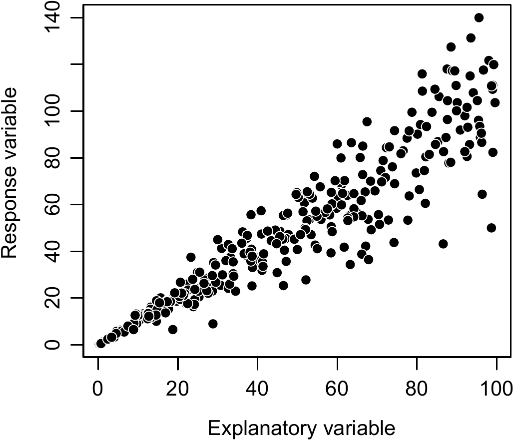
Figure 6.12: Linear relation between an effect variable (\(X\)) and a response variable (\(Y\)), with an increase in the variability of \(Y\) with an increase in \(X\) (heteroscedasticity).

As model (6.17) was fitted by simple linear regression, its sum of squares corresponds to: \[ \mathrm{SSE}(a,\ b)=\sum_{i=1}^n(Y'_i-aX'_i-b)^2 =\sum_{i=1}^n(Y_i/X_i-a/X_i-b)^2=\sum_{i=1}^nX_i^{-2}(Y_i-a-bX_i)^2 \] Here we recognize the expression for the sum of squares for a weighted regression using the weight \(w_i=X_i^{-2}\). Thus, the variable transformation \(Y'=Y/X\) and \(X'=1/X\) is strictly identical to a weighted regression of weight \(w=1/X^2\).

Red line 6.9 \(\looparrowright\) Linear regression between \(B/D^2\) and \(H\)

We saw in red line 6.5 that a double-entry biomass model using dbh and height corresponds to: \(B=a+bD^2H+\varepsilon\) where \(\mathrm{Var}(\varepsilon)\propto D^4\). By dividing each member of the equation by \(D^2\), we obtain: \[ B/D^2=a/D^2+bH+\varepsilon' \] where \[ \mathrm{Var}(\varepsilon')=\sigma^2 \] Thus, the regression of the response variable \(Y=B/D^2\) against the two effect variables \(X_1=1/D^2\) and \(X_2=H\) in principle satisfies the hypotheses of multiple linear regression. This regression is fitted by the ordinary least squares method. Fitting of this multiple regression by the command:

summary(lm((Btot / dbh^2) ~ -1 + I(1 / dbh^2) + heig, data = dat))

yields:

##             Estimate Std. Error t value Pr(>|t|)    
## I(1/dbh^2) 1.181e-03  2.288e-03   0.516    0.608    
## heig       2.742e-05  1.527e-06  17.957   <2e-16 ***

where it can be seen that the coefficient associated with \(X_1=1/D^2\) is not significantly different from zero. If we now return to the starting data, this means simply that the y-intercept \(a\) is not significantly different from zero, something we had already noted in red line 6.5. Therefore, \(X_1\) may be withdrawn and a simple linear regression may be fitted of \(Y=B/D^2\) against \(X_2=H\):

with(dat, plot(
  x = heig, 
  y = Btot / dbh^2, 
  xlab = "Height (m)", 
  ylab = "Biomass/square of dbh (t/cm2)"
  ))

m <- lm((Btot / dbh^2) ~ -1 + heig, data = dat)
summary(m)

plot(m, which = 1:2)

The scatter plot of \(B/D^2\) against \(H\) is indeed a straight line with a variance of \(B/D^2\) that is approximately constant ( Figure 6.13). Fitting the simple linear regression yields:

##       Estimate Std. Error t value Pr(>|t|)    
## heig 2.747e-05  1.511e-06   18.19   <2e-16 ***

with \(R^2=\) and a residual standard deviation of  tonnes cm^-2. The model is written: \(B/D^2=2.747\times10^{-5}H\), or if we return to the starting variables: \(B=2747\times10^{-5}D^2H\). We now need to check that this model is strictly identical to the weighted regression of \(B\) against \(D^2H\) shown in red line 6.5 with weighting proportional to \(1/D^4\). The plot of the residuals against the fitted values and the quantile-quantile plot of the residuals are shown in Figure 6.14.

Figure 6.13: Scatter plot of biomass divided by the square of the dbh (tonnes cm^-2) against height (m) for the 42 trees measured in Ghana by Henry et al. (2010).

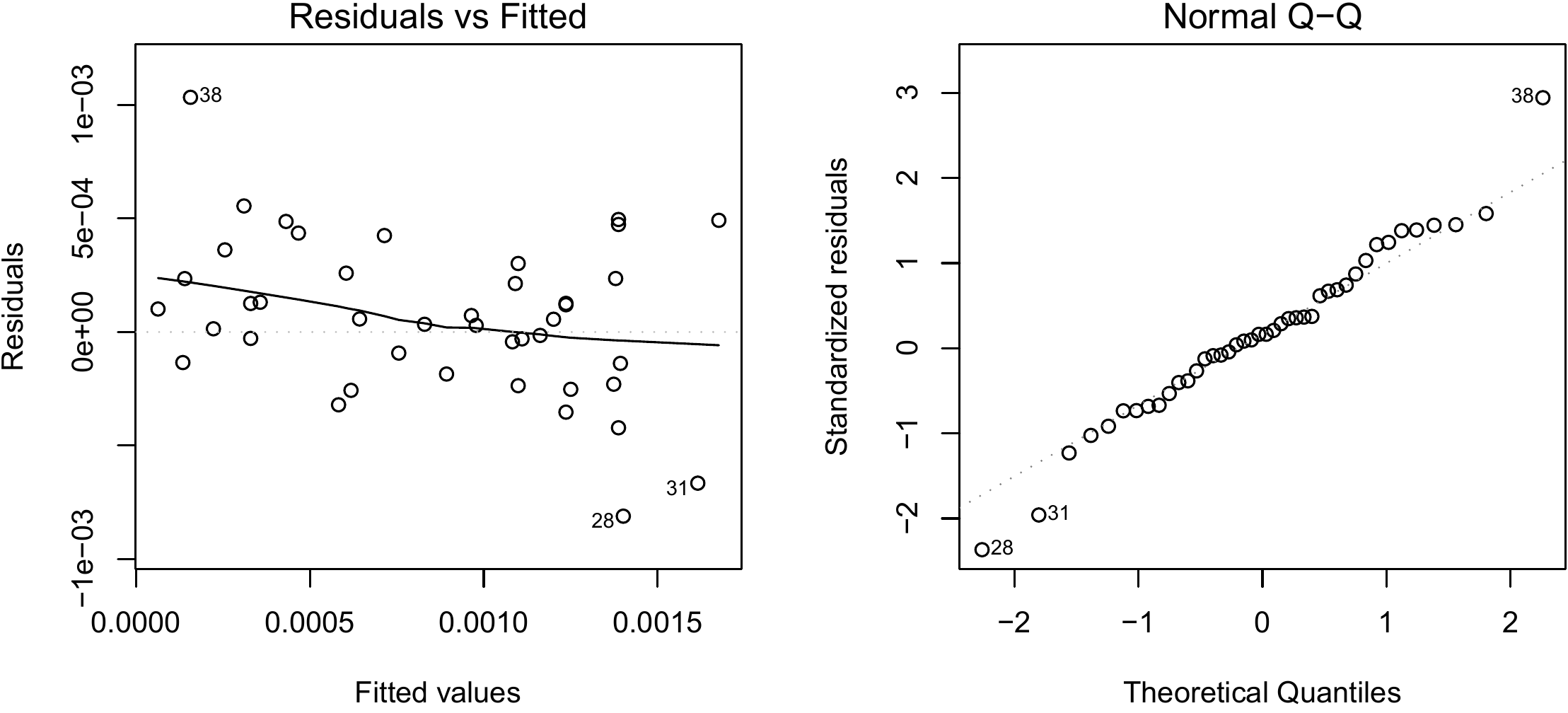
Figure 6.14: Residuals plotted against fitted values (left) and quantile–quantile plot (right) of the residuals of the simple linear regression of \(B/D^2\) against \(H\) fitted for the 42 trees measured by Henry et al. (2010) in Ghana.

Red line 6.10 \(\looparrowright\) Linear regression between \(B/D^2\) and \(1/D\)

We saw in red line @ref\(\looparrowright\) Weighted polynomial regression between \(B\) and \(D\) that a polynomial biomass model against dbh corresponded to: \(B=a_0+a_1D+a_2D^2+\varepsilon\) where \(\mathrm{Var}(\varepsilon)\propto D^4\). By dividing each member of the equation by \(D^2\), we obtain: \[ B/D^2=a_0/D^2+a_1/D+a_2+\varepsilon' \] where \[ \mathrm{Var}(\varepsilon')=\sigma^2 \] Thus, the regression of the response variable \(Y=B/D^2\) against the two effect variables \(X_1=1/D^2\) and \(X_2=1/D\) in principle satisfies the hypotheses of multiple linear regression. This regression is fitted by the ordinary least squares method. Fitting this multiple regression by the command:

summary(lm((Btot / dbh^2) ~ I(1 / dbh^2) + I(1 / dbh), data = dat))

yields:

##               Estimate Std. Error t value Pr(>|t|)    
## (Intercept)  1.215e-03  9.014e-05  13.478 2.93e-16 ***
## I(1/dbh^2)   1.127e-02  6.356e-03   1.772  0.08415 .  
## I(1/dbh)    -7.297e-03  2.140e-03  -3.409  0.00153 **

where it can be seen that the coefficient associated with \(X_1=1/D^2\) is not significantly different from zero. If we now return to the starting data, this means simply that the y-intercept \(a_0\) is not significantly different from zero, something we had already noted in red line 6.6. Therefore, \(X_1\) may be withdrawn and a simple linear regression may be fitted of \(Y=B/D^2\) against \(X_2=1/D\):

with(dat, plot(
  x = 1 / dbh, 
  y = Btot / dbh^2, 
  xlab = "1/Diameter (/cm)", 
  ylab = "Biomass/square of dbh (t/cm2)"
  ))

m <- lm((Btot / dbh^2) ~ I(1 / dbh), data = dat)
summary(m)

plot(m, which=1:2)

The scatter plot of \(B/D^2\) against \(1/D\) is approximately a straight line with a variance of \(B/D^2\) that is approximately constant (Figure 6.15). Fitting the simple linear regression yields:

##               Estimate Std. Error t value Pr(>|t|)    
## (Intercept)  1.124e-03  7.599e-05  14.789  < 2e-16 ***
## I(1/dbh)    -3.840e-03  9.047e-04  -4.245 0.000126 ***

with \(R^2=\) and a residual standard deviation of  tonnes cm^-2. The model is written: \(B/D^2=1.124\times10^{-3}-3.84\times10^{-3}D^{-1}\), or if we return to the starting variables: \(B=-3.84\times10^{-3}D+1.124\times10^{-3}D^2\). We now need to check that this model is strictly identical to the polynomial regression of \(B\) against \(D\) shown in red line 6.6 with weighting proportional to \(1/D^4\). The plot of the residuals against the fitted values and the quantile-quantile plot of the residuals are shown in Figure 6.16.

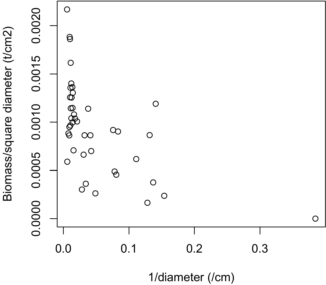
Figure 6.15: Scatter plot of biomass divided by the square of the dbh (tonnes in cm^-2) against the inverse of the dbh (cm^-1) for 42 trees measured in Ghana by Henry et al. (2010).

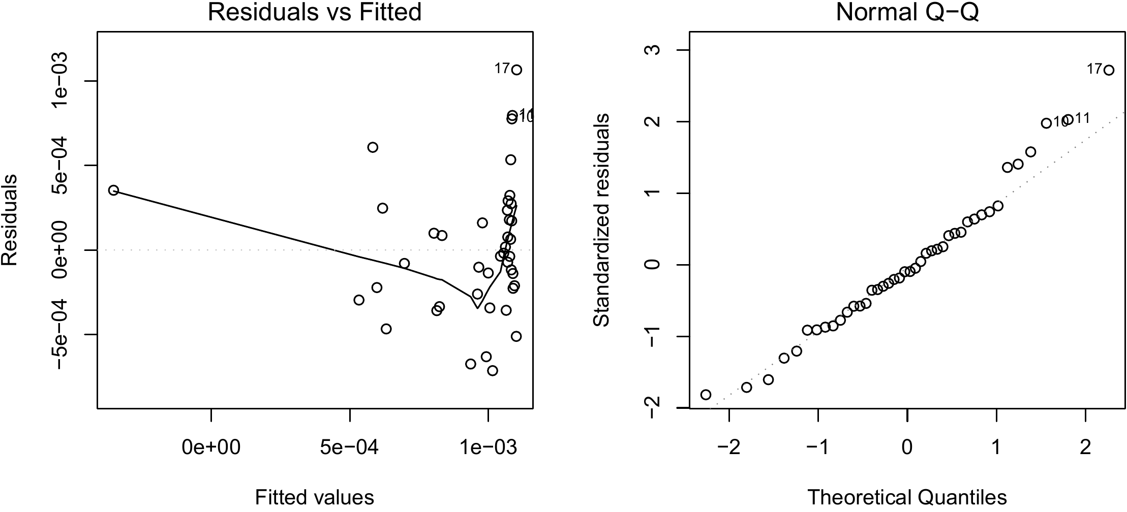
Figure 6.16: Residuals plotted against fitted values (left) and quantile–quantile plot (right) of the residuals of the simple linear regression of \(B/D^2\) against \(1/D\) fitted for the 42 trees measured by Henry et al. (2010) in Ghana.

6.2 Fitting a non-linear model

Let us now address the more general case of fitting a non-linear model. This model is written: \[ Y=f(X_1,\ \ldots,\ X_p;\theta)+\varepsilon \] where \(Y\) is the response variable, \(X_1\), \(\ldots\), \(X_p\) are the effect variables, \(\theta\) is the vector of all the model coefficients, \(\varepsilon\) is the residual error, and \(f\) is a function. If \(f\) is linear in relation to the coefficients \(\theta\), this brings us back to the previously studied linear model. We will henceforth no longer make any a priori hypotheses concerning the linearity of \(f\) in relation to coefficients \(\theta\). As previously, we assume that the residuals are independent and that they follow a centered normal distribution. By contrast, we do not make any a priori hypothesis concerning their variance. \(\mathrm{E}(\varepsilon)=0\) means that \(\mathrm{E}(Y)=f(X_1,\ \ldots,\ X_p;\theta)\). This is why we can say that \(f\) defines the mean model (i.e. for \(Y\)). Let us write: \[ \mathrm{Var}(\varepsilon)=g(X_1,\ \ldots,\ X_p;\vartheta) \] where \(g\) is a function and \(\vartheta\) a set of parameters. As \(\mathrm{Var}(Y)=\mathrm{Var}(\varepsilon)\), we can say that \(g\) defines the variance model. Function \(g\) may take various forms, but for biomass or volume data it is generally a power function of a variable that characterizes tree size (typically dbh). Without loss of generality, we can put forward that this effect variable is \(X_1\), and therefore: \[ g(X_1,\ \ldots,\ X_p;\vartheta)\equiv(kX_1^c)^2 \] where \(\vartheta\equiv(k,\ c)\), \(k>0\) and \(c\geq0\).

Interpreting the results of fitting a non-linear model is fundamentally the same as for the linear model. The difference between the linear model and the non-linear model, in addition to their properties, lies in the manner by which model coefficients are estimated. Two particular approaches are used: (i) exponent \(c\) is fixed in advance; (ii) exponent \(c\) is a parameter to be estimated in the same manner as the model’s other parameters.

6.2.1 Exponent known

Let us first consider the case where the exponent \(c\) of the variance model is known in advance. Here, the least squares method can again be used to fit the model. The weighted sum of squares corresponds to: \[ \mathrm{SSE}(\theta)=\sum_{i=1}^nw_i\ \varepsilon_i^2 =\sum_{i=1}^nw_i\ [Y_i-f(X_{i1},\ \ldots,\ X_{ip};\theta)]^2 \] where the weights are inversely proportional to the variance of the residuals: \[ w_i=\frac{1}{X_{i1}^{2c}}\propto\frac{1}{\mathrm{Var}(\varepsilon_i)} \] As previously, the estimator of the model’s coefficients corresponds to the value of \(\theta\) that minimizes the weighted sum of squares: \[ \hat{\theta}=\arg\min_{\theta}\mathrm{SSE}(\theta) =\arg\min_{\theta}\bigg\{\sum_{i=1}^n\frac{1}{X_{i1}^{2c}} [Y_i-f(X_{i1},\ \ldots,\ X_{ip};\theta)]^2\bigg\} \] In the particular case where the residuals have a constant variance (i.e. \(c=0\)), the weighted least squares method is simplified to the ordinary least squares method (all weights \(w_i\) are 1), but the principle behind the calculations remains the same. The estimator \(\theta\) is obtained by resolving \[\begin{equation} \frac{\partial\mathrm{SSE}}{\partial\theta}(\hat{\theta})=0 \tag{6.18} \end{equation}\] with the constraint \((\partial^2\mathrm{SSE}/\partial\theta^2)>0\) to ensure that this is indeed a minimum, not a maximum. In the previous case of the linear model, resolving (6.18) yielded an explicit expression for the estimator \(\hat{\theta}\). This is not the case for the general case of the non-linear model: there is no explicit expression for \(\hat{\theta}\). The sum of squares must therefore be minimized using a numerical algorithm. We will examine this point in depth in section 6.2.3.

A priori value for the exponent

The a priori value of exponent \(c\) is obtained in the non-linear case in the same manner as for the linear case : by trial and error, by dividing \(X_1\) into classes and estimating the variance of \(Y\) for each class, or by minimizing Furnival’s index .

Red line 6.11 \(\looparrowright\) Weighted non-linear regression between \(B\) and \(D\)

The graphical exploration (red lines 5.1 and 5.4) showed that the relation between biomass \(B\) and dbh \(D\) was of the power type, with the variance of the biomass increasing with dbh: \[ B=aD^b+\varepsilon \] where \[ \mathrm{Var}(\varepsilon)\propto D^{2c} \] We saw in red line 6.5 that the conditional standard deviation of the biomass derived from the dbh was proportional to the square of the dbh: \(c=2\). We can therefore fit a non-linear regression by the weighted least squares method using a weighting that is inversely proportional to \(D^4\):

start <- coef(lm(log(Btot) ~ I(log(dbh)), data =  dat[dat$Btot > 0,]))
start[1] <- exp(start[1])
names(start) <- c("a", "b")
m <- nls(
  formula = Btot ~ a * dbh^b, 
  data = dat, 
  start = start, 
  weights = 1 / dat$dbh^4
  )
summary(m)

The non-linear regression is fitted using the nls command which calls on the start values of the coefficients. These start values are contained in the start object and are calculated by re-transforming the coefficients of the linear regression on the log-transformed data. Fitting the non-linear regression by the weighted least squares method gives:

##    Estimate Std. Error t value Pr(>|t|)    
## a 2.492e-04  7.893e-05   3.157  0.00303 ** 
## b 2.346e+00  7.373e-02  31.824  < 2e-16 ***

with a residual standard deviation \(k=\) ` tonnes cm^-2. The model is therefore written: \(B=2.492\times10^{-4}D^{2.346}\). Let us now return to the linear regression fitted to log-transformed data (red line 6.1) which was written: \(\ln(B)=-8.42722+2.36104\ln(D)\). If we return naively to the starting data by applying the exponential function (we will see in § 7.2.4 why this is naive), the model becomes: \(B=\exp(-8.42722)\times D^{2.36104}=2.188\times10^{-4}D^{2.36104}\). The model fitted by non-linear regression and the model fitted by linear regression on log-transformed data are therefore very similar.

Red line 6.12 \(\looparrowright\) Weighted non-linear regression between \(B\) and \(D^2H\)

We have already fitted a power model \(B=a(D^2H)^b\) by simple linear regression on log-transformed data (red line 6.2). Let us now fit this model directly by non-linear regression: \[ B=a(D^2H)^b+\varepsilon \] where \[ \mathrm{Var}(\varepsilon)\propto D^{2c} \] In order to take account of the heteroscedasticity, and considering that the conditional standard deviation of the biomass derived from the diameter is proportional to \(D^2\) (red line 6.5), we can fit this non-linear model by the weighted least squares method using a weighting inversely proportional to \(D^4\):

start <- coef(lm(
  formula = log(Btot) ~ I(log(dbh^2 * heig)),
  data = dat[dat$Btot > 0,]
  ))
start[1] <- exp(start[1])
names(start) <- c("a", "b")
m <- nls(
  formula = Btot ~ a*(dbh^2 * heig)^b, 
  data = dat, 
  start = start, 
  weights = 1 / dat$dbh^4
  )
summary(m)

As previously (red line 6.11), the nls command calls on start values for the coefficients and these are obtained from the coefficients of the multiple regression on log-transformed data. The result of the fitting is as follows:

##    Estimate Std. Error t value Pr(>|t|)    
## a 7.885e-05  2.862e-05   2.755  0.00879 ** 
## b 9.154e-01  2.957e-02  30.953  < 2e-16 ***

with a residual standard deviation \(k=\) tonnes cm^-2. The model is therefore written: \(B=7.885\times10^{-5}(D^2H)^{0.9154}\). Let us now return to the linear regression fitted to log-transformed data (red line 6.2), which was written: \(\ln(B)=-8.99427+0.87238\ln(D^2H)\). If we return naively to the starting data by applying the exponential function, this model becomes: \(B=\exp(-8.99427)\times D^{0.87238}=1.241\times10^{-4}D^{0.87238}\). The model fitted by non-linear regression and the model fitted by linear regression on log-transformed data are therefore very similar.

Red line 6.13 \(\looparrowright\) Weighted non-linear regression between \(B\), \(D\) and \(H\)

We have already fitted a power model \(B=aD^{b_1}H^{b_2}\) by multiple linear regression on log-transformed data (red line 6.4). Let us now fit this model directly by non-linear regression: \[ B=aD^{b_1}H^{b_2}+\varepsilon \] where \[ \mathrm{Var}(\varepsilon)\propto D^{2c} \] In order to take account of the heteroscedasticity, and considering that the conditional standard deviation of the biomass derived from dbh is proportional to \(D^2\) (red line 6.5), we can fit this non-linear model by the weighted least squares method using a weighting inversely proportional to \(D^4\):

start <- coef(lm(
  log(Btot) ~ I(log(dbh)) + I(log(heig)), data = dat[dat$Btot > 0,]
  ))
start[1] <- exp(start[1])
names(start) <- c("a", "b1", "b2")
m <- nls(
  formula = Btot ~ a * dbh^b1 * heig^b2, 
  data = dat, 
  start = start, 
  weights = 1 / dat$dbh^4
  )
summary(m)

As previously (red line 6.11), the nls command calls on start values for the coefficients and these are obtained from the coefficients of the multiple regression on log-transformed data. The result of the fitting is as follows:

##     Estimate Std. Error t value Pr(>|t|)    
## a  1.003e-04  5.496e-05   1.824   0.0758 .  
## b1 1.923e+00  1.956e-01   9.833 4.12e-12 ***
## b2 7.435e-01  3.298e-01   2.254   0.0299 *

with a residual standard deviation \(k=\) tonnes cm^-2. The model is therefore written: \(B=1.003\times10^{-4}D^{1.923}H^{0.7435}\). The model is similar to that fitted by multiple regression on log-transformed data (red line 6.4). But coefficient \(a\) is estimated with less precision here than by the multiple regression on log-transformed data.

6.2.2 Estimating the exponent

Let us now consider the case where the exponent \(c\) needs to be estimated at the same time as the model’s other parameters. This case includes the linear regression with variance model that we mentioned in section 6.1.4. In this case the least squares method is no longer valid. We are therefore obliged to use another fitting method: the maximum likelihood method. The likelihood of an observation (\(X_{i1}\), \(\ldots\), \(X_{ip}\), \(Y_i\)) is the probability density of observing (\(X_{i1}\), \(\ldots\), \(X_{ip}\), \(Y_i\)) in the specified model. The probability density of a normal distribution of expectation \(\mu\) and standard deviation \(\sigma\) is: \[ \phi(x)=\frac{1}{\sigma\sqrt{2\pi}}\exp\bigg[-\frac{1}{2}\bigg( \frac{x-\mu}{\sigma}\bigg)^2\bigg] \] As \(Y_i\) follows a normal distribution of expectation \(f(X_{i1},\ \ldots,\ X_{ip};\theta)\) and standard deviation \(kX_{i1}^c\), the likelihood of the \(i\)th observation is: \[ \frac{1}{kX_{i1}^c\sqrt{2\pi}}\exp\bigg[-\frac{1}{2}\bigg( \frac{Y_i-f(X_1,\ \ldots,\ X_p;\theta)}{kX_{i1}^c}\bigg)^2\bigg] \] As the observations are independent, their joint likelihood is the product of the likelihoods of each observation. The likelihood of the sample of \(n\) observations is therefore: \[\begin{eqnarray} \ell(\theta,\ k,\ c) &=& \prod_{i=1}^n \frac{1}{kX_{i1}^c\sqrt{2\pi}}\exp\bigg[-\frac{1}{2}\bigg( \frac{Y_i-f(X_1,\ \ldots,\ X_p;\theta)}{kX_{i1}^c}\bigg)^2\bigg] \tag{6.19} \\ &=& \frac{1}{(k\sqrt{2\pi})^n}\frac{1}{(\prod_{i=1}^nX_{i1})^c} \exp\bigg[-\frac{1}{2}\sum_{i=1}^n\bigg( \frac{Y_i-f(X_1,\ \ldots,\ X_p;\theta)}{kX_{i1}^c}\bigg)^2\bigg] \nonumber \end{eqnarray}\] This likelihood is considered to be a function of parameters \(\theta\), \(k\) and \(c\).

The better the values of parameters \(\theta\), \(k\) and \(c\) the higher the probability of the observations being obtained in the model corresponding to these parameter values. In other words, the best values for parameters \(\theta\), \(k\) and \(c\) are those that maximize the likelihood of the observations. The corresponding estimator is by definition the maximum likelihood estimator, and is written: \[ (\hat{\theta},\ \hat{k},\ \hat{c})=\arg\max_{(\theta,\ k,\ c)}\; \ell(\theta,\ k,\ c)=\arg\max_{(\theta,\ k,\ c)}\; \ln[\ell(\theta,\ k,\ c)] \] where the last equality stems from the fact that a function and its logarithm reach their maximum for the same values of their argument. The logarithm of the likelihood, which we call the log-likelihood and which we write \(\mathcal{L}\), is easier to calculate than the likelihood, and therefore, for our calculations, it is the log-likelihood we will be seeking to maximize. In the present case, the log-likelihood is written: \[\begin{eqnarray} \mathcal{L}(\theta,\ k,\ c) &=& \ln[\ell(\theta,\ k,\ c)] \tag{6.20} \\ &=& -n\ln(k\sqrt{2\pi})-c\sum_{i=1}^n\ln(X_{i1})-\frac{1}{2}\sum_{i=1}^n\bigg( \frac{Y_i-f(X_1,\ \ldots,\ X_p;\theta)}{kX_{i1}^c}\bigg)^2\nonumber \\ &=& -\frac{1}{2}\sum_{i=1}^n\bigg[\bigg( \frac{Y_i-f(X_1,\ \ldots,\ X_p;\theta)}{kX_{i1}^c}\bigg)^2 +\ln(2\pi)+\ln(k^2X_i^{2c})\bigg]\nonumber \end{eqnarray}\] To obtain the maximum likelihood estimators of the parameters, we would need to calculate the partial derivatives of the log-likelihood with respect to these parameters, and look for the values where they cancel each other out (while ensuring that the second derivatives are indeed negative). In the general case, there is no analytical solution to this problem. In the same manner as previously for the sum of squares, we will need to use a numerical algorithm to maximize the log-likelihood. We can show that the maximum likelihood method yields a coefficients estimator that is asymptotically (i.e. when the number \(n\) of observations tends toward infinity) the best. We can also show that in the case of the linear model, the least squares estimator and the maximum likelihood estimator are the same.

Red line 6.14 \(\looparrowright\) Non-linear regression between \(B\) and \(D\) with variance model

Let us look again at the non-linear regression between biomass and dbh (see red line 6.11), but this time consider that exponent \(c\) in the variance model is a parameter that needs to be estimated like the others. The model is written in the same fashion as before (red line 6.11): \[ B=aD^b+\varepsilon \] where \[ \mathrm{Var}(\varepsilon)=(kD^c)^2 \] but is fitted by the maximum likelihood method:

start <- coef(lm(log(Btot) ~ I(log(dbh)), data = dat[dat$Btot > 0,]))
start[1] <- exp(start[1])
names(start) <- c("a", "b")
library(nlme)
m <- nlme(
  model = Btot ~ a * dbh^b, 
  data = cbind(dat, g = "a"), 
  fixed = a + b ~ 1,
  start = start, 
  groups = ~g, 
  weights = varPower(form = ~dbh)
  )
summary(m)

The model is fitted by the nlme command³ which, like the nls command (red line 6.11), requires start values for the coefficients. These start values are calculated as in red line 6.11. The result of the fitting is as follows:

##          Value    Std.Error DF   t-value      p-value
## a 0.0002444623 7.136164e-05 40  3.425683 1.431028e-03
## b 2.3510499658 6.947401e-02 40 33.840713 4.684925e-31

with an estimated value of exponent \(c=2.090814\). This estimated value is very similar to that evaluated for the weighted non-linear regression (\(c=2\), see in red line 6.5). The fitted model is therefore: \(B=2.445\times10^{-4}D^{2.35105}\), which is very similar to the model fitted by weighted non-linear regression (red line 6.11).

Red line 6.15 \(\looparrowright\) Non-linear regression between \(B\) and \(D^2H\) with variance model

Let us look again at the non-linear regression between biomass and \(D^2H\) (see red line 6.12), but this time consider that exponent \(c\) in the variance model is a parameter that needs to be estimated like the others. The model is written in the same fashion as before (red line 6.12): \[ B=a(D^2H)^b+\varepsilon \] where \[ \mathrm{Var}(\varepsilon)=(kD^c)^2 \] but is fitted by the maximum likelihood method:

start <- coef(lm(
  formula = log(Btot) ~ I(log(dbh^2 * heig)), 
  data = dat[dat$Btot > 0,]
  ))
start[1] <- exp(start[1])
names(start) <- c("a", "b")

library(nlme)
m <- nlme(
  model   = Btot ~ a * (dbh^2 * heig)^b, 
  data    =  cbind(dat, g = "a"),
  fixed   = a + b ~ 1, 
  start   = start, 
  groups  = ~g, 
  weights = varPower(form = ~dbh)
  )
summary(m)

The model is fitted by the nlme command, which, like the nls command (red line 6.11), requires start values for the coefficients. These start values are calculated as in red line 6.11. The result of the fitting is as follows:

##          Value    Std.Error DF   t-value      p-value
## a 0.0000819357 2.852774e-05 40  2.872142 6.492376e-03
## b 0.9122144285 2.862782e-02 40 31.864613 4.779915e-30

with an estimated value of exponent \(c=2.042586\). This estimated value is very similar to that evaluated for the weighted non-linear regression (\(c=2\), see red line 6.5). The fitted model is therefore: \(B=8.19\times10^{-5}(D^2H)^{0.9122144}\), which is very similar to the model fitted by weighted non-linear regression (red line 6.12).

Red line 6.16 \(\looparrowright\) Non-linear regression between \(B\), \(D\) and \(H\) with variance model

Let us look again at the non-linear regression between biomass, dbh and height (see red line 6.13): \[ B=aD^{b_1}H^{b_2}+\varepsilon \] where \[ \mathrm{Var}(\varepsilon)=(kD^c)^2 \] but this time consider that exponent \(c\) in the variance model is a parameter that needs to be estimated like the others. The fitting by maximum likelihood is as follows:

library(nlme)
start <- coef(lm(
  log(Btot) ~ I(log(dbh)) + I(log(heig)), data = dat[dat$Btot > 0,]
  ))
start[1] <- exp(start[1])
names(start) <- c("a", "b1", "b2")
m <- nlme(
  model   = Btot ~ a * dbh^b1 * heig^b2, 
  data    = cbind(dat, g = "a"), 
  fixed   = a + b1 + b2 ~ 1,
  start   = start, 
  groups  = ~g, 
  weights = varPower(form = ~dbh)
  )
summary(m)

and, as previously, requires the provision of start values for the coefficients. The fitting yields:

##          Value    Std.Error DF  t-value      p-value
## a  0.000110913 5.659208e-05 39 1.959868 5.718487e-02
## b1 1.943487599 1.947994e-01 39 9.976866 2.732305e-12
## b2 0.692625581 3.211766e-01 39 2.156526 3.726785e-02

with an estimated value of exponent \(c=\) 2.0555534. This estimated value is very similar to that evaluated for the weighted non-linear regression (\(c=2\), see red line 6.5). The fitted model is therefore: \(B=1.109\times10^{-4}D^{1.9434876}H^{0.6926256}\), which is very similar to the model fitted by weighted non-linear regression (red line 6.13).

Red line 6.17 \(\looparrowright\) Non-linear regression between \(B\) and a polynomial of \(\ln(D)\)

Previously (red line 6.3), we used multiple regression to fit a model between \(\ln(B)\) and a polynomial of \(\ln(D)\). If we look again at the start variable, the model is written: \[ B=\exp\{a_0+a_1\ln(D)+a_2[\ln(D)]^2+\ldots+a_p[\ln(D)]^p\}+\varepsilon \] where \[ \mathrm{Var}(\varepsilon)=(kD^c)^2 \] We will now directly fit this non-linear model by maximum likelihood (such that exponent \(c\) is estimated at the same time as the model’s other parameters). For a third-order polynomial, the fitting is obtained by:

library(nlme)
start <- coef(lm(
  log(Btot) ~ I(log(dbh)) + I(log(dbh)^2) + I(log(dbh)^3), 
  data = dat[dat$Btot > 0,]
  ))
start[1] <- exp(start[1])
names(start) <- paste("a", 0:3, sep = "")
m <- nlme(
  model = Btot ~ exp(a0 + a1 * log(dbh) + a2 * log(dbh)^2 + a3 * log(dbh)^3),
  data = cbind(dat, g = "a"), 
  fixed = a0 + a1 + a2 + a3 ~ 1,
  start = start, 
  groups = ~g, 
  weights = varPower(form = ~dbh)
  )
summary(m)

and results in:

##          Value  Std.Error DF    t-value      p-value
## a0 -8.99041010 2.29609083 38 -3.9155289 0.0003625208
## a1  2.94478161 2.11009164 38  1.3955705 0.1709459839
## a2 -0.16016443 0.61793888 38 -0.2591914 0.7968865838
## a3  0.01359927 0.05818961 38  0.2337061 0.8164676343

with an estimated value of exponent \(c=\) 2.0999225. This result is very similar to that obtained by multiple regression on log-transformed data (red line 6.3).

6.2.3 Numerical optimization

If, in the case of a non-linear model, we are looking to minimize the sum of squares (when exponent \(c\) is known) or maximize the log-likelihood (when exponent \(c\) needs to be estimated) we need to use a numerical optimization algorithm. As maximizing the log-likelihood is equivalent to minimizing the opposite of the log-likelihood, we shall, in all that follows, consider only the problem of minimizing a function in a multidimensional space. A multitude of optimization algorithms have been developed (Press et al. 2007, chapitre 10) but the aim here is not to present a review of them all. What simply needs to be recognized at this stage is that these algorithms are iterative and require parameter start values. Based on this start value and each iteration, the algorithm shifts in the parameter space while looking to minimize the target function (i.e. the sum of squares or minus the log-likelihood). The target function may be represented as a hypersurface in the parameter space (Figure 6.17). Each position in this space corresponds to a value of the parameters. A lump in this surface corresponds to a local maximum of the target function, whereas a dip in the surface corresponds to a local minimum. The aim is to determine the overall minimum, i.e. the deepest dip. The position of this dip corresponds to the estimated value of the parameters. If the algorithm gives the position of a dip that is not the deepest, the estimation of the parameters is false.

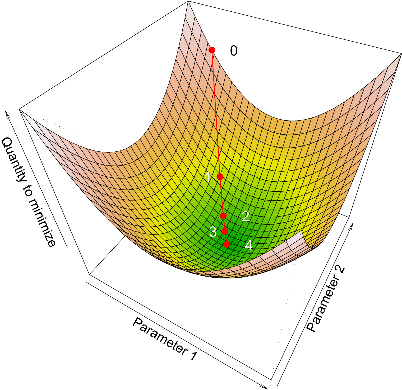
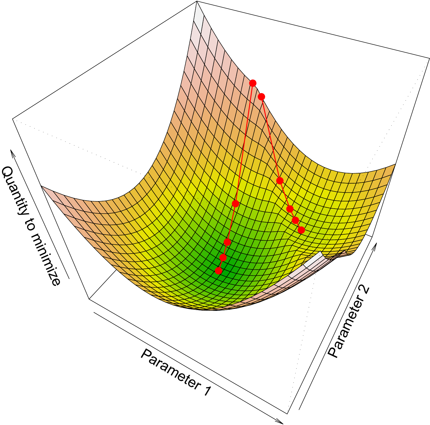
Figure 6.17: Representation of the target function (i.e. the quantity to be minimized) as a surface in parameter space. Each position in this space corresponds to a value of the parameters. The successive values \(\theta_1\), \(\theta_2\), , for the parameters are obtained from a start value \(\theta_0\) by descending the surface along the line with the steepest slope.(A) The surface has a single watershed. (B) The surface has several watersheds.

Descending algorithm

The simplest optimization algorithm consists in calculating successive positions, i.e. successive parameter values, by descending the surface defined by the target function along the line that has the steepest slope (Figure 6.17A). This algorithm leads to one dip in the surface, but nothing says that this dip is the deepest for the surface may have several watersheds with several dips. Depending on the starting position, the algorithm will converge toward one dip or another (Figure 6.17B). Also, even two starting positions very close together may be located on either side of a crest separating the two watersheds, and will therefore result in different dips, i.e. in different parameter estimations. The only case where this algorithm gives the correct parameter estimation regardless of starting value is when the surface has only a single dip, i.e. when the target function is convex. This in particular is the case for the linear model, but generally not for the non-linear model.

Improving algorithms in the case of local minima

More subtle algorithms have been developed than those descending along the steepest slope. For example, these may include the possibility to climb out of a dip into which the algorithm has temporarily converged in order to determine whether there might not be a deeper dip in the neighborhood. But no algorithm, even the most subtle, offers the certainty that it has converged to the deepest dip. Thus, any numerical optimization algorithm (i) may be trapped by a local minimum instead of converging to the overall minimum, and (ii) is sensitive to the indicated start position, which in part determines the final position toward which the algorithm will converge.

If we now return to the issue at hand, this means (i) fitting a non-linear model could yield erroneous parameter estimations, and (ii) selecting parameter start values for the algorithm is a sensitive issue. Herein lies the main drawback of fitting a non-linear model, and if it is to be avoided, the parameter start values must be carefully selected and, above all, several values must be tested.

Selecting parameter start values

When mean model \(f\) can be transformed into a linear relation between the response variable \(Y\) and the effect variables \(X_1\), \(\ldots\), \(X_p\), a start value for the coefficients may be obtained by fitting a linear regression on the transformed variables without considering the possible heteroscedasticity of the residuals. Let us for example consider a power type biomass table: \[\begin{equation} B=aD^{b_1}H^{b_2}\rho^{b_3}+\varepsilon\tag{6.21} \end{equation}\] where \[ \varepsilon\mathop{\sim}_{\mathrm{i.i.d.}}\mathcal{N}(0,\;kD^c) \] The power model for the expectation of \(B\) can be rendered linear by log-transforming the variables: \(\ln(B)=a'+b_1\ln(D)+b_2\ln(H)+b_3\ln(\rho)\). But this transformation is incompatible with the additivity of the errors in the model (6.21). In other words, the multiple regression of the response variable \(\ln(B)\) against the effect variables \(\ln(D)\), \(\ln(H)\) and \(\ln(\rho)\): \[\begin{equation} \ln(B)=a'+b_1\ln(D)+b_2\ln(H)+b_3\ln(\rho)+\varepsilon'\tag{6.22} \end{equation}\] where \(\varepsilon'\sim\mathcal{N}(0,\ \sigma)\), is not a model equivalent to (6.21), even when the residuals \(\varepsilon'\) of this model have a constant variance. Even though models (6.21) and (6.22) are not mathematically equivalent, the coefficients of (6.22) — estimated by multiple regression — may serve as start values for the numerical algorithm that estimates the coefficients of (6.21). If we write as \(x^{(0)}\) the start value of parameter \(x\) for the numerical optimization algorithm, we thus obtain: \[ a^{(0)}=\exp(\hat{a}'),\quad b_i^{(0)}=\hat{b}_i,\quad k^{(0)}=\hat{\sigma},\quad c^{(0)}=0 \] Sometimes, the mean model cannot be rendered linear. An example of this is the following biomass table used for trees in a plantation (Saint-André et al. 2005): \[ B=a+[b_0+b_1T+b_2\exp(-b_3T)]D^2H+\varepsilon \] where \(T\) is the age of the plantation and \(\varepsilon\sim\mathcal{N}(0,\ kD^c)\), which has a mean model that cannot be rendered linear. In this case, parameter start values must be selected empirically. For this current example we could for instance take: \[ a^{(0)}=\hat{a},\quad b_0^{(0)}+b_2^{(0)}=\hat{b}_0,\quad b_1^{(0)}=\hat{b}_1,\quad b_3^{(0)}=0,\quad k^{(0)}=\hat{\sigma},\quad c^{(0)}=0 \] where \(\hat{a}\), \(\hat{b}_0\), \(\hat{b}_1\) and \(\hat{\sigma}\) are estimated values for the coefficients and residual standard deviations of the multiple regression of \(B\) against \(D^2H\) and \(D^2HT\). Selecting parameter start values does not mean that several start values should not be tested. Therefore, when fitting a non-linear model with a numerical optimization algorithm, it is essential to test several parameter start values to ensure that the estimations are stable.

6.3 Selecting variables and models

When we look to construct a volume or biomass table, the graphical exploration of the data (chapter 5) generally yields several possible model forms. We could fit all these potentially interesting models, but ultimately, which of all these fitted models should be recommended to the user? Selecting variables and selecting models aims to determine which is the “best” possible expression of the model among all those fitted.

6.3.1 Selecting variables

Let us take the example of a biomass table we are looking to construct from a dataset that includes tree diameter (dbh) and height, and wood specific density. By working on log-transformed data, and given the variables they include, we may fit the following models: \[\begin{eqnarray*} \ln(B) &=& a_0+a_1\ln(D)+\varepsilon\\ % \ln(B) &=& a_0+a_2\ln(H)+\varepsilon\\ % \ln(B) &=& a_0+a_3\ln(\rho)+\varepsilon\\ % \ln(B) &=& a_0+a_1\ln(D)+a_2\ln(H)+\varepsilon\\ % \ln(B) &=& a_0+a_1\ln(D)+a_3\ln(\rho)+\varepsilon\\ % \ln(B) &=& a_0+a_2\ln(H)+a_3\ln(\rho)+\varepsilon\\ % \ln(B) &=& a_0+a_1\ln(D)+a_2\ln(H)+a_3\ln(\rho)+\varepsilon \end{eqnarray*}\] The complete model (the last in the above list) is that which includes all the effect variables available. All the other models may be considered to be subsets of the complete model, but where certain effect variables have been employed and other set aside. Selecting the variables aims to choose — from among the effect variables of the complete model — those that should be kept and those that may be set aside as they contribute little to the prediction of the response variable. In other words, in this example, selecting the variables would consist in choosing the best model from among the seven models envisaged for \(\ln(B)\).

Given that there are \(p\) effect variables \(X_1\), \(X_2\), \(\ldots\), \(X_p\), there are \(2^p-1\) models that include all or some of these effect variables. Selecting the variables consists in choosing the “best” combination of effect variables from all those available. This means firstly that we must have criterion that can be used to evaluate the quality of a model. We have already seen that \(R^2\) is a poor criterion for evaluating the quality of one model in comparison with that of another as it increases automatically with the number of effect variables, and this regardless of whether these provide information useful for predicting the response variable or not. A better criterion for selecting effect variables is the residual variance estimator, which is linked to \(R^2\) by the relation: \[ \hat{\sigma}^2=\frac{n}{n-p-1}(1-R^2)\ S_Y^2 \] where \(S_Y^2\) is the empirical variance of the response variable.

Several methods may be used to select the best combination of effect variables. If \(p\) is not too high, we can review all the \(2^p-1\) possible models exhaustively. When \(p\) is too high, a step by step method may be used to select the variables. Step-by-step methods proceed by the successive elimination or successive addition of effect variables. The descending method consists in eliminating the least significant of the \(p\) variables. The regression is then recalculated and the process repeated until a stop criterion is satisfied (e.g. when all model coefficients are significantly different from zero). The ascending method proceeds in the opposite direction: we start with the best single-variable regression and add the variable that increases \(R^2\) the most until the stop criterion is satisfied.

The so-called stepwise method is a further improvement upon the previous algorithm that consists in performing an additional Fisher’s significance test at each step such as not to introduce a non-significant variable and possibly eliminate variables that have already been introduced but are no longer informative given the last variable selected. The algorithm stops when no more variables can be added or withdrawn. The different step-by-step selection methods do not necessarily give the same result, but the “stepwise” method would appear to be the best. They do not, however, safeguard from the untimely removal of variables that are actually significant, which may well bias the result. And in connection with this, it should be recalled that if we know (for biological reasons) why a variable should be included in a model (e.g. wood specific density), it is not because a statistical test declares it non-significant that it should be rejected (because of the test’s type II error).

Red line 6.18 \(\looparrowright\) Selecting variables

Let us select the variables \(\ln(D)\), \([\ln(D)]^2\), \([\ln(D)]^3\), \(\ln(H)\) to predict the log of the biomass. The complete model is therefore: \[ \ln(B)=a_0+a_1\ln(D)+a_2[\ln(D)]^2+a_3[\ln(D)]^3+a_4\ln(H) +\varepsilon \] where \[ \mathrm{Var}(\varepsilon)=\sigma^2 \] Variables are selected in R using the step command applied to the fitted complete model:

m <- lm(
  formula = log(Btot) ~ I(log(dbh))+I(log(dbh)^2)+I(log(dbh)^3)+I(log(heig)),
  data = dat[dat$Btot>0,]
  )
summary(step(m))

which yields:

##               Estimate Std. Error t value Pr(>|t|)    
## (Intercept)   -6.50202    0.35999 -18.062  < 2e-16 ***
## I(log(dbh)^2)  0.23756    0.01972  12.044 1.53e-14 ***
## I(log(heig))   1.01874    0.17950   5.675 1.59e-06 ***

The variables selected are therefore \([\ln(D)]^2\) and \(\ln(H)\). The model finally retained is therefore: \(\ln(B)=-6.50202+0.23756[\ln(D)]^2+1.01874\ln(H)\), with a residual standard deviation of and \(R^2=\) .

6.3.2 Selecting models

Given two competitor models that predict the same response variable to within one transformation of a variable, which should we choose? Let us look at a few different cases before answering this question.

Nested models

The simplest case is where the two models to be compared are nested. A model is nested in another if the two predict the same response variable and if we can move from the second to the first by removing one or several effect variables. For example, the biomass table \(B=a_0+a_1D+\varepsilon\) is nested in \(B=a_0+a_1D+a_2D^2H+\varepsilon\) since we can move from the second to the first by deleting \(D^2H\) from the effect variables. Likewise, the model \(B=a_0+a_2D^2H+\varepsilon\) is nested in \(B=a_0+a_1D+a_2D^2H+\varepsilon\) since we can move from the second to the first by deleting \(D\) from the effect variables. By contrast, the model \(B=a_0+a_1D+\varepsilon\) is not nested in \(B=a_0+a_2D^2H+\varepsilon\). Let \(p\) be the number of effect variables in the complete model and \(p'<p\) be the number of effect variables in the nested model. Without loss of generality, we can write the complete model as: \[\begin{equation} Y=f(X_1,\ \ldots,\ X_{p'},\ X_{p'+1},\ \ldots,\ X_p; \theta_0,\ \theta_1)+\varepsilon\tag{6.23} \end{equation}\] where (\(\theta_0\), \(\theta_1\)) is the vector of the coefficients associated with the complete model and \(\theta_0\) is the vector of the coefficients associated with the nested model, which may be obtained by setting \(\theta_1=\mathbf{0}\). In the particular case of the linear model, the complete model is obtained as the sum of the nested model and additional terms: \[\begin{equation} \underbrace{\underbrace{Y=a_0+a_1X_1+\ldots+a_{p'}X_{p'}}_{\scriptsize \mbox{nested model}}+ a_{p'+1}X_{p'+1}+\ldots+a_pX_p}_{\scriptsize \mbox{complete model}}+\varepsilon\tag{6.24} \end{equation}\] where \(\theta_0=(a_0,\ \ldots,\ a_{p'})\) and \(\theta_1=(a_{p'+1},\ \ldots,\ a_p)\).

In the case of nested models, a statistical test can be used to test one of the models against the other. The null hypothesis of this test is that \(\theta_1=\mathbf{0}\), i.e. the additional terms are not significant, which can also be expressed as: the nested model is better than the complete model. If the p-value of this test proves to be below the significance level (typically 5 %), then the null hypothesis is rejected, i.e. the complete model is best. Conversely, if the p-value is above the significance threshold, the nested model is considered to be the best.

In the case of the linear model (6.24), the test statistic is a ratio of the mean squares, which under the null hypothesis follows Fisher’s distribution. This is the same type of test as that used to test the overall significance of a multiple regression, or that used in the “stepwise” method of selecting variables. In the general case of the non-linear model (6.23), the test statistic is a likelihood ratio, such that \(-2\log\)(likelihood ratio) under the null hypothesis follows a \(\chi^2\) distribution.

Red line 6.19 \(\looparrowright\) Testing nested models: \(\ln(D)\)

In red line 6.18 the variable \([\ln(D)]^2\) was selected with \(\ln(H)\) as effect variable of \(\ln(B)\) but not \(\ln(D)\). Model \(\ln(B)=a_0+a_1\ln(D)+a_2[\ln(D)]^2+a_4\ln(H)\), which includes the additional term \(\ln(D)\), can be compared with the model \(\ln(B)=a_0+a_2[\ln(D)]^2+a_4\ln(H)\) using the nested models test. In R, the anova command can be used to test a nested model, with the first argument being the nested model and the second being the complete model:

comp <- lm(
  formula = log(Btot) ~ I(log(dbh)) + I(log(dbh)^2) + I(log(heig)), 
  data = dat[dat$Btot > 0,]
  )
nest <- lm(
  formula = log(Btot) ~ I(log(dbh)^2) + I(log(heig)), 
  data=dat[dat$Btot > 0,]
  )
anova(nest, comp)

The test gives the following result:

##   Res.Df    RSS Df Sum of Sq      F Pr(>F)
## 1     38 6.0605                           
## 2     37 5.8964  1   0.16407 1.0295 0.3169

The p-value is , therefore greater than 5 %. The nested model (without \(\ln(D)\)) is therefore selected rather than the complete model.

Red line 6.20 \(\looparrowright\) Testing nested models: \(\ln(H)\)

The model \(\ln(B)=-8.42722+2.36104\ln(D)\) was obtained in red line 6.1 whereas red line 6.4 gave the model \(\ln(B)=-8.9050+1.8654\ln(D)+0.7083\ln(H)\). As the first is nested in the second, we can test for which is the best. The command

comp <- lm(
  formula = log(Btot) ~ I(log(dbh)) + I(log(heig)), 
  data = dat[dat$Btot > 0,]
  )
nest <- lm(
  formula = log(Btot) ~ I(log(dbh)), 
  data = dat[dat$Btot > 0,]
  )
anova(nest, comp)

yields:

##   Res.Df    RSS Df Sum of Sq     F   Pr(>F)   
## 1     39 8.3236                               
## 2     38 6.4014  1    1.9222 11.41 0.001698 **

As the p-value is less than 5 %, the complete model (including \(\ln(H)\) as effect variable) is selected rather than the nested model.

Models with the same response variable

When we want to compare two models that have the same response variable but are not nested, we can no longer use a statistical test. For example, we cannot use the above-mentioned test to compare \(B=a_0+a_1D+\varepsilon\) and \(B=a_0+a_2D^2H+\varepsilon\). In this case, we must use an information criterion (Bozdogan 1987; Burnham and Anderson 2002, 2004). There are several, suited to different contexts. The most widespread are the “Bayesian information criterion”, or BIC, and above all the Akaike (1974) information criterion (or AIC). The AIC is expressed as: \[ \mathrm{AIC}=-2\ln\ell(\hat{\theta})+2q \] where \(\ell(\hat{\theta})\) if the model’s likelihood, i.e. the likelihood of the sample for the values estimated from model parameters, see equation (6.19), and \(q\) is the number of free parameters estimated. In particular, in the case of a multiple regression against \(p\) effect variables, \(q=p+1\) (i.e. the \(p\) coefficients associated with the \(p\) effect variables plus the y-intercept). The coefficient \(-2\) in front of the log-likelihood in the AIC expression is identical to that in the test statistic on the likelihood ratio in the case of nested models. Given two models with the same number of parameters, the best model is that with the highest likelihood, therefore that with the smallest AIC. At equal likelihoods, the best model is that with the fewest parameters (in accordance with the principle of Occam’s razor), and therefore is once more that with the smallest AIC. When all is said and done, the best model is that with the smallest value of AIC.

The BIC is similar in expression to the AIC, but with a term that penalizes more strongly the number of parameters: \[ \mathrm{BIC}=-2\ln\ell(\hat{\theta})+q\ln(n) \] where \(n\) is the number of observations. Here again, the best model is that with the smallest value of BIC. When fitting volume or biomass tables, AIC is used rather than BIC as a model selection criterion.

Red line 6.21 \(\looparrowright\) Selecting models with \(B\) as response variable

The following models with B as response variable were fitted:

• red line 6.6 or 6.10: \(B=-3.840\times10^{-3}D+1.124\times10^{-3}D^2\)
• red line 6.8: \(B=-3.319456\times10^{-3}D+1.067068\times10^{-3}D^2\)
• red line 6.11: \(B=2.492\times10^{-4}D^{2.346}\)
• red line 6.14: \(B=2.445\times10^{-4}D^{2.35105}\)
• red line 6.5 or 6.9: \(B=2.747\times10^{-5}D^2H\)
• red line 6.7: \(B=2.740688\times10^{-5}D^2H\)
• red line 6.12: \(B=7.885\times10^{-5}(D^2H)^{0.9154}\)
• red line 6.15: \(B=8.19\times10^{-5}(D^2H)^{0.9122144}\)
• red line 6.13: \(B=1.003\times10^{-4}D^{1.923}H^{0.7435}\)
• red line 6.16: \(B=1.109\times10^{-4}D^{1.9434876}H^{0.6926256}\)

The models in red lines 6.6, 6.8, 6.5 and 6.7 are fitted by linear regression while the others are fitted by non-linear regression. These models have five distinct forms, with two fitting methods for each: using a weighted regression by the weighted least squares method (red lines 6.6, 6.11, 6.5, 6.12 and 6.13) or using a regression with variance model by the maximum likelihood method (red lines 6.8, 6.14, 6.7, 6.15 and 6.16). The predictions made by these different models are shown in Figure 6.18. Let m be one of the fitted models with dbh as the only entry. A plot of the predictions made by this model may be obtained as follows:

## model (red line 14)
m <-  lm(
  formula = Btot ~ dbh + I(dbh^2), 
  data = dat, 
  weights = 1/dat$dbh^4
  )
with(dat, plot(x = dbh, y = Btot, xlab = "Dbh (cm)", ylab = "Biomass (t)"))
D <- seq(par("usr")[1], par("usr")[2], length=200)
lines(D, predict(m, newdata = data.frame(dbh = D)), col = "red")

For a model m that has dbh and height as entries, its predictions may be obtained as follows:

## model (red line 22)
library(nlme)
start <- coef(lm(
  log(Btot) ~ I(log(dbh)) + I(log(heig)), data = dat[dat$Btot > 0,]
  ))
start[1] <- exp(start[1])
names(start) <- c("a", "b1", "b2")
m <- nlme(
  model   = Btot ~ a * dbh^b1 * heig^b2,
  data    = cbind(dat, g = "a"),
  fixed   = a + b1 + b2 ~ 1,
  start   = start,
  groups  = ~g,
  weights = varPower(form = ~dbh)
  )

## Predictions
D <- seq(0,180,length=20)
H <- seq(0,61,length=20)
newdata <- data.frame(expand.grid(dbh=D, heig=H), g = "a")
B <- matrix(predict(m, newdata), length(D))

and a plot of the biomass response surface against diameter and height may be obtained by:

M <- persp(
  x = D, y = H, z = B, 
  xlab = "Dbh (cm)", ylab = "Height (m)", zlab="Biomass (t)", 
  ticktype = "detailed", theta = -30, phi = 20
  )
points(trans3d(x = dat$dbh, y = dat$heig, z = dat$Btot, pmat = M))

Given a fitted model m, its AIC may be calculated by the command:

AIC(m)

AIC values for the 10 models listed above are given in Table 6.1. This table illustrates a problem that arises with several statistical software packages, including R: when we maximize the log-likelihood (6.20), the constants (such as \(-n\ln(2\pi)/2\)) no longer play any role. The constant we use to calculate the log-likelihood, and by consequence AIC, is therefore a matter of convention, and different constants are used depending on the calculation. Thus, in Table 6.1, we can see that the values of AIC in models fitted by the nls command are substantially higher than those in the other models: it is not that these models are substantially worse than the others, it is simply that the nls command uses a constant different from the others to calculate the log-likelihood. Therefore, with R, it should be remembered that the values of AIC should be compared only for models that have been fitted using the same command. In our present case, if we compare the two models that were fitted with the lm command, the best (i.e. that with the smallest AIC) is that which has \(D^2H\) as effect variable (red line 6.5). If we compare the five models fitted with the nlme command, the best is again that with \(D^2H\) as effect variable (red line 6.7). And if we compare the three models fitted with the nls command, the best is yet again that with \(D^2H\) as effect variable (red line 6.12). It may therefore be concluded that whatever fitting method is used, the biomass table that uses \(D^2H\) as effect variable is the best.

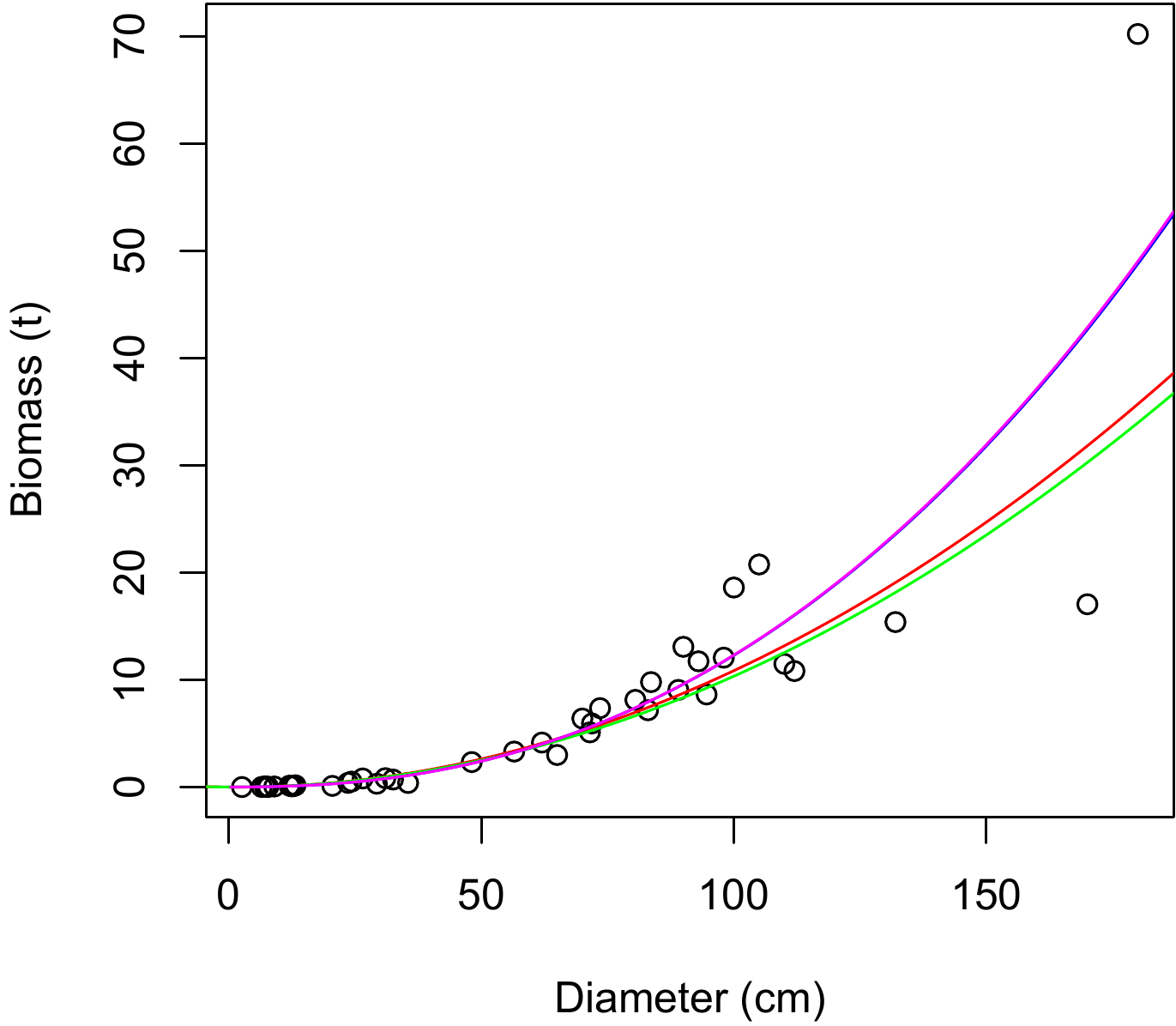
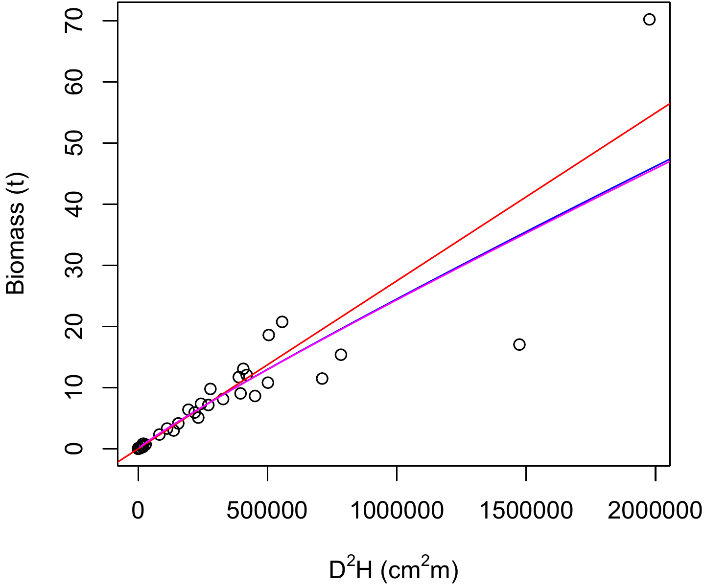
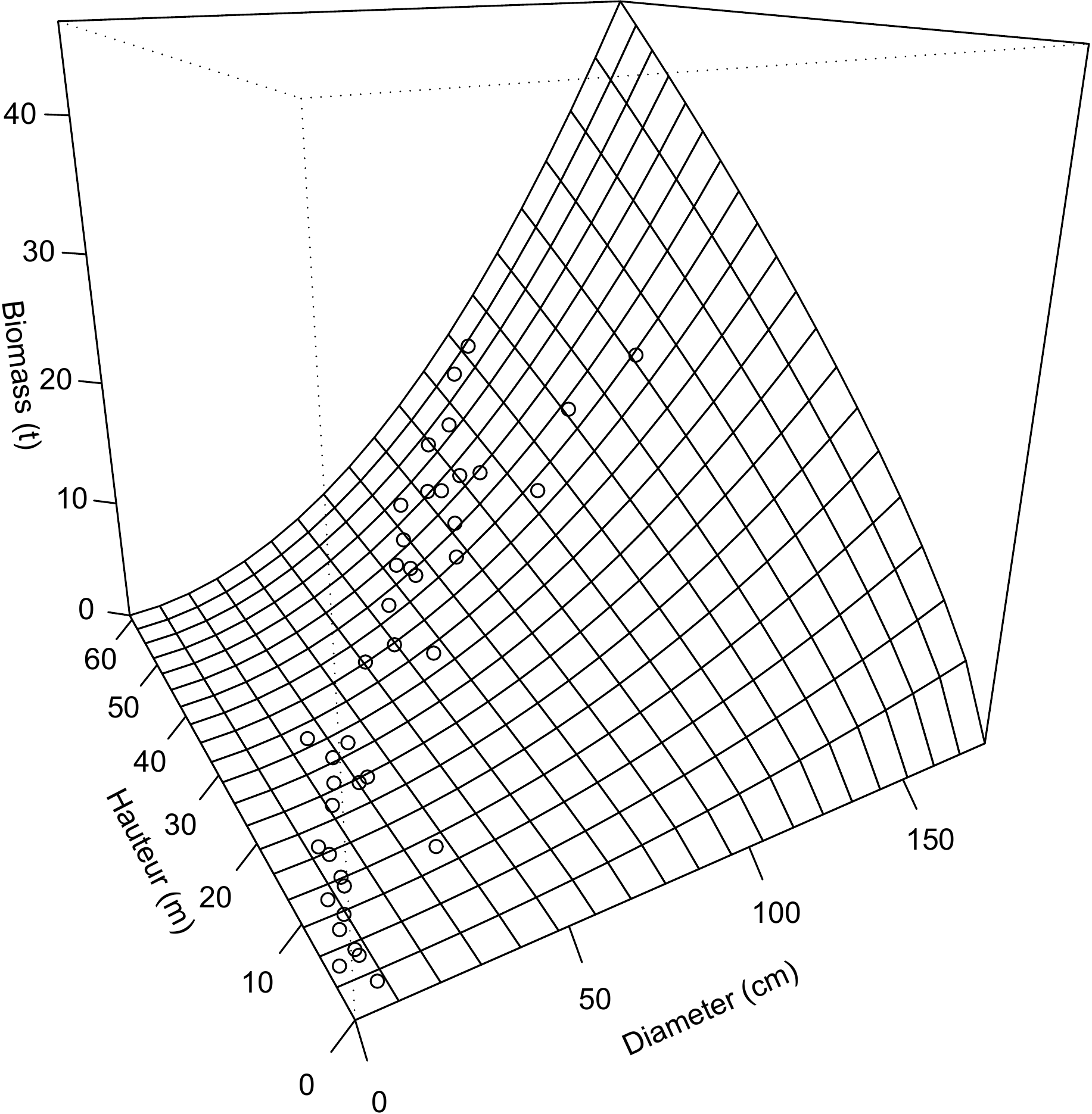
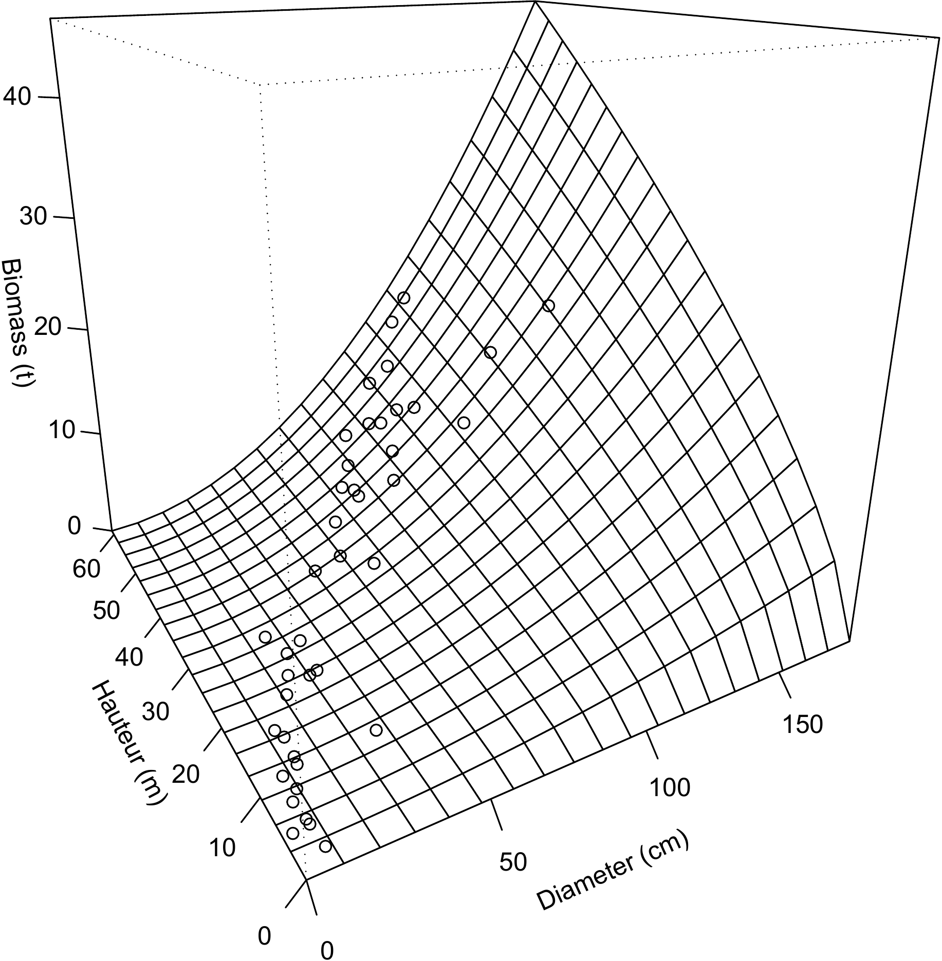
Figure 6.18: Biomass predictions by different tables fitted to data from 42 trees measured in Ghana by Henry et al. (2010). The data are shown as points. (A) Tables with dbh as only entry, corresponding to red lines 6.6 (red), 6.8 (green), 6.11 (blue) and 6.14 (magenta). (B) Tables with \(D^2H\) as the only effect variable, corresponding to red lines 6.5 (red), 6.7 (green), 6.12 (blue) and 6.15 (magenta). (C) Table corresponds to red line 6.13. (D) Table corresponds to red line 6.16.

Table 6.1: AIC values for 10 biomass tables fitted to data from 42 trees measured in Ghana by Henry et al. (2010). These 10 tables directly predict biomass.

Red line	Entry	Fitting\(^*\) method	R command	AIC
6.6	\(D\)	WLS	lm	76.71133
6.8	\(D\)	ML	nlme	83.09157
6.11	\(D\)	WLS	nls	24809.75727
6.14	\(D\)	ML	nlme	75.00927
6.5	\(D^2H\)	WLS	lm	65.15002
6.7	\(D^2H\)	ML	nlme	69.09644
6.12	\(D^2H\)	WLS	nls	24797.53706
6.15	\(D^2H\)	ML	nlme	69.24482
6.13	\(D\), \(H\)	WLS	nls	24802.91248
6.16	\(D\), \(H\)	ML	nlme	76.80204
* WLS = weighted least squares, ML = maximum likelihood

Red line 6.22 \(\looparrowright\) Selecting models with \(\ln(B)\) as response variable

The following models with \(\ln(B)\) as response variable were fitted:

• red line 6.1 or 6.3: \(\ln(B)=-8.42722+2.36104\ln(D)\)
• red line 6.2: \(\ln(B)=-8.99427+0.87238\ln(D^2H)\)
• red line 6.4: \(\ln(B)=-8.9050+1.8654\ln(D)+0.7083\ln(H)\)
• red line 6.18: \(\ln(B)=-6.50202+0.23756[\ln(D)]^2+1.01874\ln(H)\)

All these models were fitted using linear regression by the ordinary least squares method. A plot of the predictions on a log scale for model m with dbh as only entry may be obtained by the following command:

## Model (red line 7)
m <- lm(log(Btot) ~ I(log(dbh)), data = dat[dat$Btot > 0,])

with(dat[dat$Btot > 0,], plot(
  x = dbh, y = Btot, xlab = "Dbh (cm)", ylab = "Biomass (t)", log = "xy"
  ))
D <- 10^par("usr")[1:2]
lines(D, exp(predict(m, newdata = data.frame(dbh = D))))

For a model that uses both dbh and height as entries, a plot on a log scale may be obtained by the command:

## Model (red line 10)
m <- lm(log(Btot) ~ I(log(dbh)) + I(log(heig)), data = dat[dat$Btot > 0,]) 

D <- exp(seq(log(1), log(180), length = 20))
H <- exp(seq(log(1), log(61), length = 20))
B <- matrix(predict(m, newdata = expand.grid(dbh = D, heig = H)), length(D))
M <- persp(
  x = log(D), y = log(H), z = B, 
  xlab="log(Diameter) (cm)",ylab="log(height) (m)", zlab="log(Biomass) (t)", 
  ticktype = "detailed", theta = -30, phi = 20
  )
points(trans3d(log(dat$dbh), log(dat$heig), log(dat$Btot), M))

Predictions of \(\ln(B)\) by the four models are given in Figure 6.19. Given a fitted model m, its AIC may be calculated by the command:

AIC(m)

## [1] 45.96998

Table 6.2 gives AIC values for the four models. As all four models were fitted by the same lm command, the AIC values are directly comparable. The best model, i.e. that with the smallest AIC, is the fourth (red line 6.18). It should also be noted that an AIC-based classification of these models is entirely consistent with the results of the nested models tests performed previously (red lines 6.19 and 6.20).

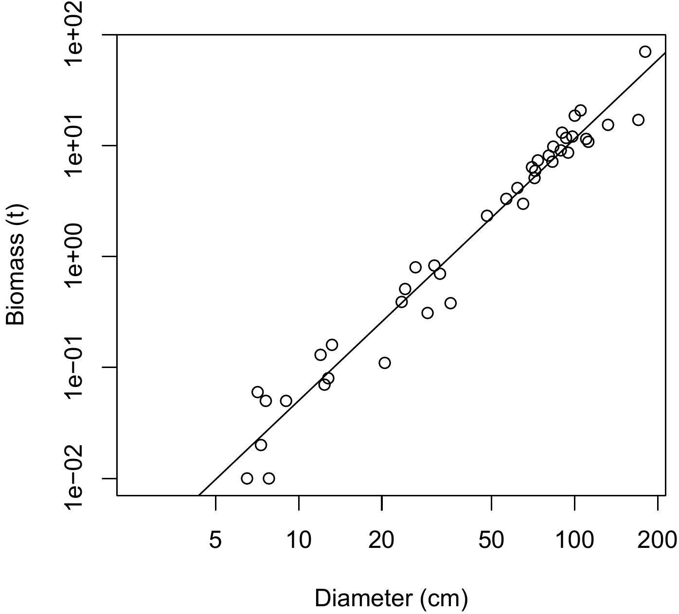
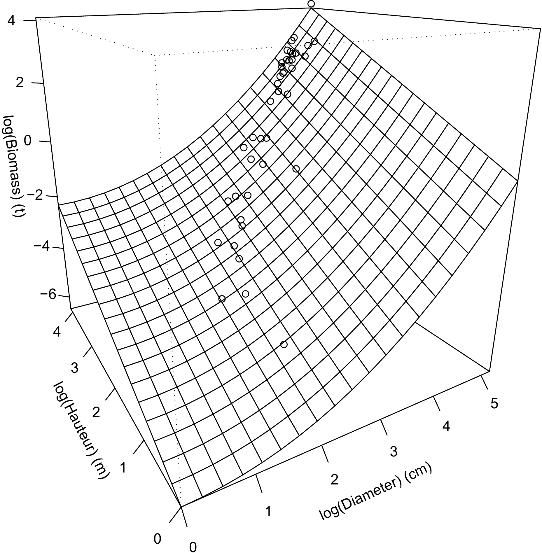
Figure 6.19: Biomass predictions by different tables fitted to data from 42 trees measured in Ghana by Henry et al. (2010). The data are shown as points. (A) Model in red line 6.1. (B) Model in red line 6.2. (C) Model in red line 6.4. (D) Model in red line 6.18.

Table 6.2: AIC values for four biomass tables fitted to data from 42 trees measured in Ghana by Henry et al. (2010). These four tables predict the log of the biomass and are all fitted using linear regression by the ordinary least squares (OLS) method.

Red line	Entry	Fitting method	R command	AIC
6.1	\(D\)	OLS	lm	56.97923
6.2	\(D^2H\)	OLS	lm	46.87780
6.4	\(D\), \(H\)	OLS	lm	48.21367
6.18	\(D\), \(H\)	OLS	lm	45.96998

Models with different response variables

The more general case is when we want to compare two models that do not have the same response variable because one is a transform of the other. For example, the models \(B=aD^b+\varepsilon\) and \(\ln(B)=a+b\ln(D)+\varepsilon\) both predict biomass, but the response variable is \(B\) in one case and \(\ln(B)\) in the other. In this case, we cannot use the AIC or BIC to compare the models. By contrast, Furnival (1961) index can in this case be used to compare the models. The model with the smallest Furnival’s index is considered to be the best (Parresol 1999).

Furnival’s index is defined only for a model whose residual error \(\varepsilon\) has a variance that is assumed to be constant: \(\mbox{Var}(\varepsilon)=\sigma^2\). By contrast, no constraint is imposed on the form of the transformation of the variable linking the modeled response variable \(Y\) to the variable of interest (volume or biomass). Let us consider the case of a biomass model (that can immediately be transposed into a volume model) and let \(\psi\) be this variable transformation: \(Y=\psi(B)\). Furnival’s index is defined by: \[ F=\frac{\hat{\sigma}}{\sqrt[n]{\prod_{i=1}^n\psi'(B_i)}} =\exp\Big(-\frac{1}{n}\sum_{i=1}^n\ln[\psi'(B_i)]\Big)\ \hat{\sigma} \] where \(\hat{\sigma}\) if the estimation of the residual standard deviation of the fitted model and \(B_i\) is the biomass of the \(i\)th tree measured. When there is no transformation of variables, \(\psi\) is the identity function and Furnival’s index \(F\) is then equal to the residual standard deviation \(\hat{\sigma}\). The most common variable transformation is the log transformation: \(\psi(B)=\ln(B)\) and \(\psi'(B)=1/B\), in which case Furnival’s index is: \[ F_{\ln}=\hat{\sigma}\sqrt[n]{\textstyle\prod_{i=1}^nB_i} =\exp\Big(\frac{1}{n}\sum_{i=1}^n\ln(B_i)\Big)\ \hat{\sigma} \] For linear regressions where the residual variance is assumed to be proportional to a power of an effect variable \(X_1\), a trick can nevertheless be used to define Furnival’s index. The linear regression: \[\begin{equation} Y=a_0+a_1X_1+a_2X_2+\ldots+a_pX_p+\varepsilon\tag{6.25} \end{equation}\] where \(\mbox{Var}(\varepsilon)=(kX_1^c)^2\); is strictly identical to the linear regression: \[\begin{equation} Y'=a_0X_1^{-c}+a_1X_1^{1-c}+a_2X_2X_1^{-c}+\ldots+ a_pX_pX_1^{-c}+\varepsilon'\tag{6.26} \end{equation}\] where \(Y'=YX_1^{-c}\), \(\varepsilon'=\varepsilon X_1^{-c}\) and \(\mbox{Var}(\varepsilon')=k^2\). As model (6.26) has constant residual variance, its Furnival’s index is defined. By extension, we can define the Furnival index of model (6.25) as being the Furnival index of model (6.26). If \(Y=\psi(B)\), then \(Y'=X_1^{-c}\psi(B)\), such that Furnival’s index is: \[ F=\frac{\hat{k}}{\sqrt[n]{\prod_{i=1}^nX_{i1}^{-c}\psi'(B_i)}} =\exp\Big(\frac{1}{n}\sum_{i=1}^n\{c\ln(X_{i1})-\ln[\psi'(B_i)]\} \Big)\ \hat{k} \] Therefore, Furnival’s index can be used to select the value of exponent \(c\) in a weighted regression.

6.3.3 Choosing a fitting method

Let us return to the method used to fit a volume or biomass model. Many solutions may be available to fit a model. Let us for instance consider the biomass model: \[ B=a\rho^{b_1}D^{b_2}H^{b_3}+\varepsilon \] where \[ \varepsilon\sim\mathcal{N}(0,\ kD^c) \] This model could be adjusted as a non-linear model (i) by the weighted least squares method (\(c\) fixed in advance) or (ii) by the maximum likelihood method (\(c\) not fixed in advance). If we apply a log transformation to the data, we could (iii) fit the multiple regression: \[ \ln(B)=a'+b_1\ln(\rho)+b_2\ln(D)+b_3\ln(H)+\varepsilon \] where \[ \varepsilon\sim\mathcal{N}(0,\ \sigma) \] Thus, for a given model that predicts biomass as a power of effect variables, we have three possible fitting methods. Obviously, methods (i)–(ii) and (iii) are based on different hypotheses concerning the structure of the residual errors: additive error with regard to \(B\) in cases (i) and (ii), multiplicative error with regard to \(B\) in case (iii). But both these error types reflect data heteroscedasticity, and therefore fitting methods (i), (ii) and (iii) all have a chance of being valid.

As another example, let us consider the biomass table: \[ B=\exp\{a_0+a_1\ln(D)+a_2[\ln(D)]^2+a_3[\ln(D)]^3+a_4\ln(\rho)\}+\varepsilon \] where \[ \varepsilon\sim\mathcal{N}(0,\ kD^c) \] Here again, we can (i) fit a non-linear model by the least squares method (specifying \(c\) in advance), (ii) fit a non-linear model by the maximum likelihood method (estimating \(c\)), or (ii) fit a multiple regression on log-transformed data: \[ \ln(B)=a_0+a_1\ln(D)+a_2[\ln(D)]^2+a_3[\ln(D)]^3+a_4\ln(\rho)+\varepsilon \] where \[ \varepsilon\sim\mathcal{N}(0,\ \sigma) \] Here again, the structure of the errors is not the same in the three cases, but all can correctly reflect the heteroscedasticity of the biomass. In most cases, the different fitting methods give very similar results in terms of predictions. Should any doubt persist regarding the most appropriate fitting method, then model selection methods may be employed to decide. But in practice the choice of a particular fitting method results rather from the importance given to the respective advantages and drawbacks of each method. Multiple regression has the drawback of imposing constraints on the form of the residuals, and has less flexibility for the mean model. By contrast, it has the advantage of offering an explicit expression for the estimators of the model’s coefficients: there is therefore no risk of having erroneous estimators for the coefficients. The non-linear model has the advantage of not imposing any constraints on the mean model or the variance model. Its drawback is that it does not have an explicit expression for parameter estimators: there is therefore the risk of having erroneous parameter estimators.

Red line 6.23 \(\looparrowright\) Power model fitting methods

We have already taken a look at three methods for fitting the power model \(B=aD^b\):

1. using a simple linear regression on log-transformed data (red line 6.1): \(\ln(B)=-8.42722+2.36104\ln(D)\), if we “naively” apply the exponential inverse transformation;

2. using a weighted non-linear regression (red line 6.11): \(B=2.492\times10^{-4}D^{2.346}\);

3. using a non-linear regression with variance model (red line 6.14): \(B=2.445\times10^{-4}D^{2.35105}\).

The predictions given by these three fittings of the same model are illustrated in Figure 6.20. The differences can be seen to be minimal and well below prediction precision, as we will see later ( 7.2).

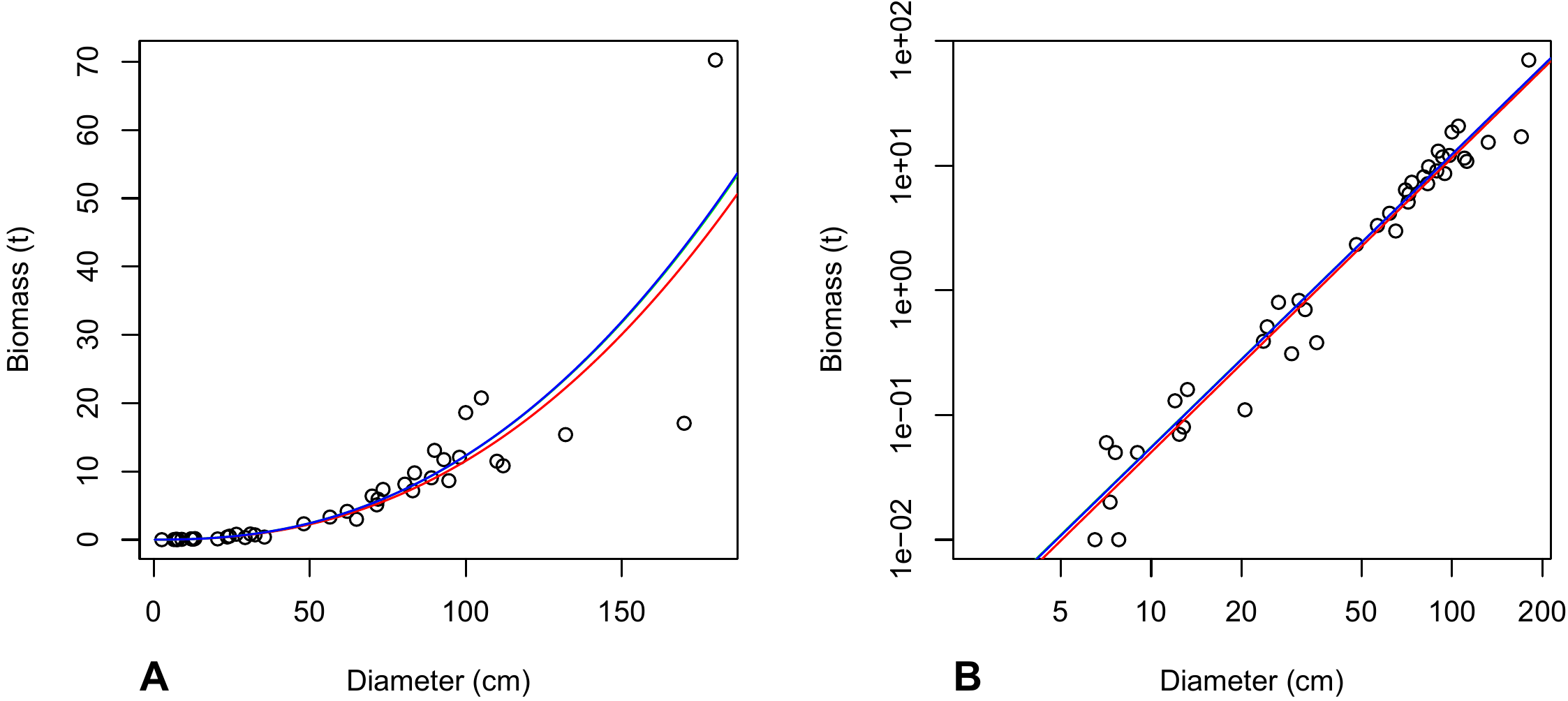
Figure 6.20: Biomass predictions by the same power table fitted in three different ways to data from 42 trees measured in Ghana by Henry et al. (2010). The data are shown as points. The red line is the linear regression on log-transformed data (red line 6.1). The green line (practically superimposed by the blue line) is the fitting by weighted non-linear regression (red line 6.11). The blue color shows the fitting by non-linear regression with variance model (red line 6.14). (A) No data transformation. (B) On a log scale.

6.4 Stratification and aggregation factors

Up until now we have considered that the dataset used to fit the volume or biomass model is homogeneous. In reality, the dataset may be drawn from measurements made under different conditions, or may have been generated by merging several separate datasets. Covariables are generally used to describe this dataset heterogeneity. For example, a covariable may indicate the type of forest in which the measurements were made (deciduous, semi-deciduous, evergreen, etc.), the type of soil, or year planted (if a plantation), etc. A crucial covariable for multispecific data is tree species. Initially, all these covariables that can explain the heterogeneity of a dataset were considered as qualitative variables (or factors). The various modalities of these factors define strata, and a well constituted dataset is one that is sampled in relation to previously identified strata (see § 2.2.3). How can these qualitative covariables be taken into account in a volume or biomass model? Is it valid to analyze the dataset in an overall manner? Or should we analyze the data subsets corresponding to each stratum separately? These are the questions we will be addressing here (§ 6.4.1).

Also, biomass measurements are made separately for each compartment in the tree (see chapter 3). Therefore, in addition to an estimation of its total biomass, we also have, for each tree in the sample, an estimation of the biomass of its foliage, the biomass of its truck, of its large branches, of its small branches, etc. How can we take account of these different compartments when establishing biomass models? We will also be addressing this question (§ 6.4.2).

6.4.1 Stratifying data

Let us now consider that there are qualitative covariables that stratify the dataset into \(S\) strata. As each stratum corresponds to a cross between the modalities of the qualitative covariables (in the context of experimental plans we speak of treatment rather than stratum) we will not consider each covariable separately. For example, if one covariable indicates the type of forest with three modalities (let us say: deciduous forest, semi-deciduous forest and evergreen forest) and another covariable indicates the type of soil with three modalities (let us say: sandy soil, clay soil, loamy soil), the cross between these two covariables gives \(S=3\times 3=9\) strata (deciduous forest on sandy soil, deciduous forest on clay soil, etc.). We are not looking to analyze the forest type effect separately, or the soil type effect separately. Also, if certain combinations of the covariable modalities are not represented in the dataset, this reduces the number of strata. For example, if there are no evergreen forests on loamy soil, the number of strata \(S=8\) instead of 9.

Therefore, when stratifying a dataset, one strategy consists in fitting a model separately for each stratum. In the case of a multiple regression, this would be written: \[ Y_s=a_{0s}+a_{1s}X_{1s}+a_{2s}X_{2s}+\ldots+a_{ps}X_{ps}+\varepsilon_s \] where \[ \varepsilon_s\mathop{\sim}_{\mathrm{i.i.d.}}\mathcal{N}(0,\ \sigma_s) \] where (\(Y_s\), \(X_{1s}\), \(\ldots\), \(X_{ps}\)) designates an observation relative to stratum \(s\), for \(s=1\), \(\ldots\), \(S\). There are now \(S\times(p+1)\) coefficients to be estimated. An alternative strategy consists in analyzing the dataset as a whole, by fitting a model such as: \[\begin{equation} Y_s=a_{0s}+a_{1s}X_{1s}+a_{2s}X_{2s}+\ldots+a_{ps}X_{ps}+\varepsilon \tag{6.27} \end{equation}\] where \[ \varepsilon\mathop{\sim}_{\mathrm{i.i.d.}}\mathcal{N}(0,\ \sigma) \] This model differs only in the structure of the error. This type of model is called an analysis of covariance. It assumes that all the residuals have the same variance, not only within each stratum, but also from one stratum to another. An analysis of covariance can test whether there is a stratum effect on the response variable, alone or in interaction with each of the effect variables \(X_1\), \(\ldots\), \(X_p\). Testing the main effect of the stratification is equivalent to testing the null hypothesis \(a_{01}=a_{02}=\ldots=a_{0S}\). The test statistic is a mean squares ratio which, under the null hypothesis, follows Fisher’s distribution. Testing the effect of the interaction between the stratification and the \(j\)th effect variable is equivalent to testing the null hypothesis \(a_{j1}=a_{j2}=\ldots=a_{jS}\). As previously, the test statistic is a mean squares ratio which, under the null hypothesis, follows Fisher’s distribution.

The advantage of testing these effects is that each time one proves not to be significant, the \(S\) coefficients \(a_{j1}\), \(a_{j2}\), \(\ldots\), \(a_{jS}\) to be estimated can be replaced by a single common coefficient \(a_j\). Let us imagine, for example, that in analysis of covariance (6.27), the main effect of the stratum is not significant, and neither is the interaction between the stratum and the first \(p'\) effect variables (where \(p'<p\)). In this case the model to be fitted is: \[ Y_s=a_0+a_1X_{1s}+\ldots+a_{p'}X_{p's}+a_{p'+1,s}X_{p'+1,s}+\ldots+a_{ps}X_{ps}+\varepsilon \] where \(\varepsilon\sim\mathcal{N}(0,\ \sigma)\). This model now includes “only” \(p'+1+(p-p')S\) coefficients to be estimated, instead of \((p+1)S\) coefficients if we fit the model separately for each stratum. As all the observations serve to estimate common coefficients \(a_0\), \(\ldots\), \(a_{p'}\), these are estimated more precisely than if we fit the model separately for each stratum.

This principle of an analysis of covariance can be immediately extended to the case of a non-linear model. Here again, we can test whether or not the coefficients are significantly different between the strata, and if necessary estimate a common coefficient for all the strata.

Red line 6.24 \(\looparrowright\) Specific biomass model

In red line 6.2, we used simple linear regression to fit a power model with \(D^2H\) as effect variable to log-transformed data: \(\ln(B)=a+b\ln(D^2H)\). We can now include species-related information in this model to test whether the coefficients \(a\) and \(b\) differ from one species to another. The model corresponds to an analysis of covariance: \[ \ln(B_s)=a_s+b_s\ln(D_s^2H_s)+\varepsilon \] where \[ \mathrm{Var}(\varepsilon)=\sigma^2 \] where index \(s\) designates the species. This model is fitted by the command:

m <- lm(
  formula = log(Btot) ~ species * I(log(dbh^2 * heig)), 
  data = dat[dat$Btot > 0,]
  )

To test whether the coefficients \(a\) and \(b\) differ from one species to another, we can use the command:

anova(m)

which yields:

##                              Df  Sum Sq Mean Sq   F value    Pr(>F)    
## species                      15 117.667   7.844   98.4396 1.647e-13 ***
## I(log(dbh^2 * heig))          1 112.689 112.689 1414.1228 < 2.2e-16 ***
## species:I(log(dbh^2 * heig))  7   0.942   0.135    1.6879    0.1785    
## Residuals                    17   1.355   0.080

The first line in the table tests for a species effect, i.e. whether the y-intercept \(a_s\) differs from one species to another. The null hypothesis of this test is that there is no difference between species: \(a_1=a_2=\ldots=a_S\), where \(S=16\) is the number of species. The test statistic is given in the “F value” column. As the p-value of the test is less than 5 %, it may be concluded that the y-intercept of the model is significantly different from one species to another. The second line in the table tests for an effect of the \(D^2H\), variable, i.e. whether the mean slope associated with this variable is significantly different from zero. The third line in the table tests whether the slope-species interaction is significant, i.e. whether slope \(b_s\) differs from one species to another. The null hypothesis is that there is no difference between species: \(b_1=b_2=\ldots=b_S\). The p-value here is 0.1785, therefore greater than 5 %: there is therefore no significant slope difference between the species.

This leads us to fit the following model: \[\begin{equation} \ln(B_s)=a_s+b\ln(D_s^2H_s)+\varepsilon\tag{6.28} \end{equation}\] which considers that slope \(b\) is the same for all species. The relevant command is:

m <- lm(
  formula = log(Btot) ~ species + I(log(dbh^2 * heig)),
  data = dat[dat$Btot > 0,]
  )
anova(m)

and yields:

##                      Df  Sum Sq Mean Sq F value    Pr(>F)    
## species              15 117.667   7.844   81.99 < 2.2e-16 ***
## I(log(dbh^2 * heig))  1 112.689 112.689 1177.81 < 2.2e-16 ***
## Residuals            24   2.296   0.096

Model coefficients may be obtained by the command:

summary(m)

which yields:

##                                  Estimate Std. Error t value Pr(>|t|)    
## (Intercept)                       -9.0036     0.4514  -19.94   <2e-16 ***
## speciesAubrevillea kerstingii     -0.5463     0.4378   -1.25    0.224    
## speciesCecropia peltata           -0.7769     0.3626   -2.14    0.043 *  
## speciesCeiba pentandra            -0.7084     0.3805   -1.86    0.075 .  
## speciesCola nitida                -0.4643     0.4448   -1.04    0.307    
## speciesDaniellia thurifera         0.0469     0.4641    0.10    0.920    
## speciesDialium aubrevilliei       -0.1563     0.4376   -0.36    0.724    
## speciesDrypetes chevalieri         0.0495     0.4539    0.11    0.914    
## speciesGarcinia epunctata          1.0965     0.4732    2.32    0.029 *  
## speciesGuarea cedrata             -0.4525     0.3846   -1.18    0.251    
## speciesHeritiera utilis           -0.2686     0.3266   -0.82    0.419    
## speciesNauclea diderrichii        -0.5546     0.3576   -1.55    0.134    
## speciesNesogordonia papaverifera  -0.4782     0.4434   -1.08    0.292    
## speciesPiptadeniastrum africanum  -0.1796     0.3572   -0.50    0.620    
## speciesStrombosia glaucescens      0.0633     0.3960    0.16    0.874    
## speciesTieghemella heckelii       -0.0910     0.3391   -0.27    0.791    
## I(log(dbh^2 * heig))               0.8998     0.0262   34.32   <2e-16 ***

The last line in this table gives the value of the slope: \(b=0.89985\). The other lines give y-intercept values for the 16 species. By convention, R proceeds in the following manner when specifying these values: the first line in the table gives the y-intercept for the first species in alphabetical order. As the first species in alphabetical order is Afzelia bella, the y-intercept for Afzelia bella is therefore \(a_1=-9.00359\). The subsequent lines give the difference \(a_s-a_1\) between the y-intercepts of the species indicated and the y-intercept of Afzelia bella. Thus, the y-intercept of Aubrevillea kerstingii is: \(a_2=a_1-0.54634=-9.00359-0.54634=-9.54993\). Finally, the expression for the specific table corresponds to: \[ \ln(B)=0.89985\ln(D^2H)-\left\{ \begin{array}{lcl} 9.00359 && \textrm{for } \textit{Afzelia bella} \\ % 9.54993 && \textrm{for } \textit{Aubrevillea kerstingii} \\ % 9.78047 && \textrm{for } \textit{Cecropia peltata} \\ % 9.71200 && \textrm{for } \textit{Ceiba pentandra} \\ % 9.46786 && \textrm{for } \textit{Cola nitida} \\ % 8.95674 && \textrm{for } \textit{Daniellia thurifera} \\ % 9.15985 && \textrm{for } \textit{Dialium aubrevilliei} \\ % 8.95406 && \textrm{for } \textit{Drypetes chevalieri} \\ % 7.90713 && \textrm{for } \textit{Garcinia epunctata} \\ % 9.45614 && \textrm{for } \textit{Guarea cedrata} \\ % 9.27223 && \textrm{for } \textit{Heritiera utilis} \\ % 9.55823 && \textrm{for } \textit{Nauclea diderrichii} \\ % 9.48176 && \textrm{for } \textit{Nesogordonia papaverifera}\\ % 9.18315 && \textrm{for } \textit{Piptadeniastrum africanum}\\ % 8.94026 && \textrm{for } \textit{Strombosia glaucescens} \\ % 9.09462 && \textrm{for } \textit{Tieghemella heckelii} \\ % \end{array} \right. \]

For a given diameter and height, the species with the highest biomass is Garcinia epunctata while that with the lowest biomass is Cecropia peltata. The model’s residual standard deviation is \(\hat{\sigma}=0.3093\) and \(R^2=0.9901\).

Case of a numerical covariable

Up until now we have considered that the covariables defining the stratification are qualitative factors. But in certain cases these covariables can also be interpreted as numerical variables. For instance, let us consider a biomass model for plantations (Saint-André et al. 2005). The year the plantation was set up (or, which comes to the same thing, the age of the trees), may be used as a stratification covariable. This year or age may be seen indifferently as a qualitative variable (cohort of trees of the same age) or as a numerical value. More generally, any numerical variable may be seen as a qualitative variable if it is divided into classes. In the case of age, we could also consider plantations aged 0 to 5 years as a stratum, plantations aged 5 to 10 years as another stratum, plantations aged 10 to 20 years as a third stratum, etc.. The advantage of dividing covariable \(Z\) into classes and considering it as a qualitative variable is that this allows us to model the relation between \(Z\) and response variable \(Y\) without any a priori constraint on the form of this relation. By contrast, if we consider \(Z\) to be a numerical variable, we are obliged a priori to set the form of the relation between \(Y\) and \(Z\) (linear relation, polynomial relation, exponential relation, power relation, etc.). The disadvantage of dividing \(Z\) into classes and considering this covariable as being qualitative is that the division introduces an element of randomness. Also, the covariance model that uses classes of \(Z\) (qualitative covariables) will generally have more parameters that need to be estimated than the model that considers \(Z\) to be a numerical covariable.

It is customary in modeling to play on this dual interpretation of numerical variables. When covariable \(Z\) is numerical (e.g. tree age), it is advisable to proceed in two steps (as explained in § 5.1.1):

1. consider \(Z\) as a qualitative variable (if necessary after division into classes) and fit a covariance model which will provide a picture of the form of the relation between Z and the model’s coefficients;

2. model this relation using an appropriate expression then return to the fitting of a linear or non-linear model, but considering \(Z\) to be a numerical variable.

If we return to the example of the age of the trees in a plantation: let us assume that age \(Z\) has been divided into \(S\) age classes. The first step consists typically of an analysis of covariance (assuming that the model has been rendered linear): \[ Y_s=a_{0s}+a_{1s}X_{1s}+a_{2s}X_{2s}+\ldots+a_{ps}X_{ps}+\varepsilon \] where \(s=1\), \(\ldots\), \(S\). Let \(Z_s\) be the median age of age class \(s\). We then draw scatter plots of \(a_{0s}\) against \(Z_s\), \(a_{1s}\) against \(Z_s\), \(\ldots\), \(a_{ps}\) against \(Z_s\) and for each scatter plot we look for the form of the relation that fits the plot. Let us imagine that \(a_{0s}\) varies in a linear manner with \(Z_s\), that \(a_{1s}\) varies in a exponential manner with \(Z_s\), that \(a_{2s}\) varies in a power manner with \(Z_s\), and that the coefficients \(a_{3s}\) to \(a_{ps}\) do not vary in relation to \(Z_s\) (which besides can be formally tested). In this particular case we will then, as the second step, fit the following non-linear model: \[ Y=\underbrace{b_0+b_1Z}_{a_{0s}}+\underbrace{b_2\exp(-b_3Z)}_{a_{1s}}X_1 +\underbrace{b_4Z^{b_5}}_{a_{2s}}X_2+a_3X_3+\ldots+a_pX_p+\varepsilon \] where age \(Z\) is now considered as a numerical variable. Such a model involving a numerical effect covariable is called a parameterized model (here by age).

Ordinal covariables warrant a special remark. An ordinal variable is a qualitative variable that establishes an order. For example, the month of the year is a qualitative variable that establishes a chronological order. The type of soil along a soil fertility gradient is also an ordinal variable. Ordinal variables are generally treated as fully fledged qualitative variables, but in this case the order information they contain is lost. An alternative consists in numbering the ordered modalities of the ordinal variable using integers, then considering the ordinal variable as a numerical variable. For example, in the case of the months of the year, we can set January = 1, February = 2, etc. This approach is meaningful only if the differences between the integers correctly reflect the differences between the modalities of the ordinal variable. For instance, if we set 1 = January 2011 up to 12 = December 2011, we will set 1 = January 2012 if the response is cyclically seasonal, whereas we will set 13 = January 2012 if the response presents as a continuous trend. In the case of three soil types along a fertility gradient, we will set 1 = poorest soil, 2 = soil of intermediate fertility, and 3 = richest soil if we consider the fertility difference between two soils induces a response that is proportional to this difference, but we will set 1 = poorest soil, 4 = soil of intermediate fertility, and 9 = richest soil if we consider that the response is proportional to the square of the fertility difference.

Special case of the species

In the case of multispecific datasets, the species is a stratification covariable that warrants special attention. If the dataset includes only a few species (less than about 10), and there are sufficient observations per species (see § 2.2.1), then species may be considered to be a stratification covariable like any other. The model in this case would be divided into \(S\) specific models, or the models could be grouped together based on the allometric resemblance of the species.

If the dataset contains many species, or if only a few observations are available for certain species, it is difficult to treat the species as a stratification covariable. A solution in this case consists in using species functional traits. Functional traits are defined here, a little abusively, as the numerical variables that characterize the species (Dı́az and Cabido 1997; Rösch, Van Rooyen, and Theron 1997; Lavorel and Garnier 2002; see Violle et al. 2007 for a more rigorous definition). The most widely used trait in biomass models is wood density. If we decide to use functional traits to represent species, these traits intervene as effect variables in the model in the same way as the effect variables that characterize the tree, for example its dbh or height. The single-entry (dbh) monospecific biomass model of the power type, which in its linear form may be written: \[ \ln(B)=a_0+a_1\ln(D)+\varepsilon \] will thus, in the multispecific case, become a double-entry biomass model: \[ \ln(B)=a_0+a_1\ln(D)+a_2\ln(\rho)+\varepsilon \] if we decide to use wood density \(\rho\) to represent the specific effect.

Red line 6.25 \(\looparrowright\) Specific wood density-dependent biomass model

In red line 6.24, species-related information was taken into account in the model \(\ln(B)=a+b\ln(D^2H)\) through a qualitative covariable. We can now capture this information through specific wood density \(\rho\). The fitted model is therefore: \[\begin{equation} \ln(B)=a_0+a_1\ln(D^2H)+a_2\ln(\rho)+\varepsilon\tag{6.29} \end{equation}\] where \[ \mathrm{Var}(\varepsilon)=\sigma^2 \] As wood density in the dataset was measured for each individual, we must start by calculating mean wood density for each species:

dm <- tapply(dat$dens, dat$species, mean)
dat2 <- cbind(dat, dmoy = dm[as.character(dat$species)])

The dat2 dataset now contains an additional variable dmoy that gives specific wood density. The model is fitted by the command:

m <- lm(
  formula = log(Btot) ~ I(log(dbh^2 * heig)) + I(log(dmoy)), 
  data = dat2[dat2$Btot > 0,]
  )
summary(m)

which yields:

##                      Estimate Std. Error t value Pr(>|t|)    
## (Intercept)          -8.38900    0.26452 -31.714  < 2e-16 ***
## I(log(dbh^2 * heig))  0.85715    0.02031  42.205  < 2e-16 ***
## I(log(dmoy))          0.72864    0.17720   4.112 0.000202 ***

with a residual standard deviation of and \(R^2=\) . The model is therefore written: \(\ln(B)=-8.38900+0.85715\ln(D^2H)+0.72864\ln(\rho)\). Is it better to take account of the species through wood density, as we have just done, or by constructing specific models as in red line 6.24? To answer this question we need to compare model (6.28) to the model (6.29) using the AIC:

AIC(m)

which yields \(\mathrm{AIC}=34.17859\) for specific model (6.28) and \(\mathrm{AIC}=33.78733\) for the model (6.29) that uses wood density. The latter therefore is slightly better, but the difference in AIC is nevertheless minor.

To better take account of wood density variations within a tree, it is possible to analyze inter- and intra-specific variations rather than use a mean density based on the hypothesis that wood density is the same from the pith to the bark and from the top to the bottom of trees (see chapter 1). Wood density can be modeled by taking account of factors such as species, functional group, tree dimensions, and radial or vertical position in the tree. An initial comparison may be made using Friedman’s analysis of variance test, followed by Tuckey’s highly significant difference (HSD) test. These tests will indicate the variables that most influence wood density. This wood density may then be modeled based on these variables (Henry et al. 2010).

Red line 6.26 \(\looparrowright\) Individual wood density-dependent biomass model

In red line 6.25, wood density \(\rho\) was defined for the species by calculating the mean of individual densities for trees in the same species. Let us now fit a biomass model based on individual wood density measurements in order to take account of inter-individual variations in wood density in a given species. The fitted model is: \[ \ln(B)=a_0+a_1\ln(D)+a_2\ln(\rho)+\varepsilon \] where \[ \mathrm{Var}(\varepsilon)=\sigma^2 \] where \(\rho\) unlike in red line 6.25, is here the individual measurement of wood density. The model is fitted by the command:

m <- lm(log(Btot) ~ I(log(dbh)) + I(log(dens)), data = dat[dat$Btot > 0,])
summary(m)

which yields:

##              Estimate Std. Error t value Pr(>|t|)    
## (Intercept)  -7.76644    0.20618 -37.668  < 2e-16 ***
## I(log(dbh))   2.35272    0.04812  48.889  < 2e-16 ***
## I(log(dens))  1.00717    0.14053   7.167 1.46e-08 ***

with a residual standard deviation of and \(R^2=\) . The model is written: \(\ln(B)=-7.76644+2.35272\ln(D)+1.00717\ln(\rho)\). According to this model, biomass is dependent upon individual wood density by the term \(\rho^{1.00717}\), i.e. practically \(\rho\). By way of a comparison, model (6.29) was dependent upon specific wood density by the term \(\rho^{0.72864}\). From a biological standpoint, the exponent 1.00717 is more satisfactory than the exponent 0.72864 since it means that the biomass is the product of a volume (that depends solely on tree dimensions) and a density. The difference between the two exponents may be attributed to inter-individual variations in wood density within the species. But the model based on individual wood density has little practical usefulness as it would require a wood density measurement in every tree whose biomass we are seeking to predict.

6.4.2 Tree compartments

Tree biomass is determined separately for each compartment in the tree (stump, trunk, large branches, small branches, leaves, etc.). Total above-ground biomass is the sum of these compartments. The approach already presented for fitting a model could be followed for each compartment separately. In this case we would construct a model for leaf biomass, a model for the biomass of the large branches, etc.. This approach integrates dataset stratification. Thus, we could initially fit a model for each compartment and each stratum; as a second step, and depending on the differences found between strata, we could aggregate the strata and/or parameterize the model in order to construct a model by compartment for all the strata. But the approach would not end there. We could also continue the data integration in order to move toward a smaller number of more integrating models.

Compartment additivity

As total above-ground biomass is the sum of the biomasses of the different compartments, it could be imagined that the best model for predicting above-ground biomass is the sum of the models predicting the biomass of each compartment. In fact, because of the correlations between the biomasses of the different compartment, this is not the case (Cunia and Briggs 1984, 1985a; Parresol 1999). Also, certain model families are not stable by addition. This in particular is the case for power models: the sum of two power functions is not a power function. If we have fitted a power model for each compartment: \[\begin{eqnarray*} B^{\mathrm{stump}} &=& a_1D^{b_1} \\ B^{\mathrm{trunk}} &=& a_2D^{b_2} \\ B^{\mathrm{large\ branches}} &=& a_3D^{b_3} \\ B^{\mathrm{small\ branches}} &=& a_4D^{b_4} \\ B^{\mathrm{leaves}} &=& a_5D^{b_5} \end{eqnarray*}\] The sum \(B^{\textrm{above-ground}}=B^{\mathrm{stump}} +B^{\mathrm{trunk}}+B^{\mathrm{large\ branches}} +B^{\mathrm{small\ branches}}+B^{\mathrm{leaves}}\) = \(\sum_{m=1}^5a_m\) \(D^{b_m}\) is not a power function of dbh. By contrast, polynomial models are stable by addition.

Fitting a multivariate model

In order to take account of the correlations between the biomasses of the different compartments, we can fit the models relative to the different compartments in a simultaneous manner rather than separately. This last step in model integration requires us to redefine the response variable. As we are looking to predict simultaneously the biomasses of different compartments, we are no longer dealing with a response variable but a response vector \(\mathbf{Y}\). The length of this vector is equal to the number \(M\) of compartments. For example, if the response variable is the biomass, \[ \mathbf{Y}=\left[ \begin{array}{l} B^{\textrm{above-ground}}\\ % B^{\mathrm{stump}}\\ % B^{\mathrm{trunk}}\\ % B^{\mathrm{large\ branches}}\\ % B^{\mathrm{small\ branches}}\\ % B^{\mathrm{leaves}} \end{array} \right] \] If the response variable is the log of the biomass, \[ \mathbf{Y}=\left[ \begin{array}{l} \ln(B^{\textrm{above-ground}})\\ % \ln(B^{\mathrm{stump}})\\ % \ln(B^{\mathrm{trunk}})\\ % \ln(B^{\mathrm{large\ branches}})\\ % \ln(B^{\mathrm{small\ branches}})\\ % \ln(B^{\mathrm{leaves}}) \end{array} \right] \] Let \(Y_m\) be the response variable of the \(m\)th compartment (where \(m=1\), \(\ldots\), \(M\)). Without loss of generality, we can consider that all the compartments have the same set \(X_1\), \(X_2\), \(\ldots\), \(X_p\) of effect variables (if a variable is not included in the prediction of a compartment, the corresponding coefficient can simply be set at zero). A model that predicts a response vector rather than a response variable is a multivariate model. An observation used to fit a multivariate model consists of a vector (\(Y_1\), \(\ldots\), \(Y_M\), \(X_1\), \(\ldots\), \(X_p\)) of length \(M+p\). The residual of a multivariate model is a vector \(\boldsymbol{\varepsilon}\) of length \(M\), equal to the difference between the observed response vector and the predicted response vector.

The expression of an \(M\)-variate model differs from the \(M\) univariate models corresponding to the different compartments only by the structure of the residual error; the structure of the mean model does not change. Let us consider the general case of a non-linear model. If the \(M\) univariate models are: \[\begin{equation} Y_m=f_m(X_1,\ \ldots,\ X_p;\theta_m)+\varepsilon_m\tag{6.30} \end{equation}\] for \(m=1\), \(\ldots\), \(M\), then the multivariate model is written: \[ \mathbf{Y}=\mathbf{F}(X_1,\ \ldots,\ X_p;\boldsymbol{\theta})+ \boldsymbol{\varepsilon} \] where \(\mathbf{Y}={}^{\mathrm{t}}{[Y_1,\ \ldots,\ Y_M]}\), \(\boldsymbol{\theta}={}^{\mathrm{t}}{[\theta_1,\ \ldots,\ \theta_M]}\), and \[\begin{equation} \mathbf{F}(X_1,\ \ldots,\ X_p;\boldsymbol{\theta})=\left[ \begin{array}{c} f_1(X_1,\ \ldots,\ X_p;\theta_1) \\\vdots\\ f_m(X_1,\ \ldots,\ X_p;\theta_m) \\\vdots\\ f_M(X_1,\ \ldots,\ X_p;\theta_M) \end{array} \right]\tag{6.31} \end{equation}\] The residual vector \(\boldsymbol{\varepsilon}\) now follows a centered multinormal distribution, with a variance-covariance matrix of: \[ \mathrm{Var}(\boldsymbol{\varepsilon})\equiv\boldsymbol{\Sigma} =\left[ \begin{array}{cccc} \sigma_1^2 & \zeta_{12} & \cdots & \zeta_{1M}\\ % \zeta_{21} & \sigma_2^2 & \ddots & \vdots\\ % \vdots & \ddots & \ddots & \zeta_{M-1,M}\\ % \zeta_{M1} & \cdots & \zeta_{M,M-1} & \sigma_M^2 \end{array} \right] \] Matrix \(\boldsymbol{\Sigma}\) is symmetrical with \(M\) lines and \(M\) columns, such that \(\sigma_m^2=\mathrm{Var}(\varepsilon_m)\) is the residual variance of the biomass of the \(m\)th compartment and \(\zeta_{ml}=\zeta_{lm}\) is the residual covariance between the biomass of the \(m\)th compartment and that of the \(l\)th compartment. Like in the univariate case, two residuals corresponding to two different observations are assumed to be independent: \(\boldsymbol{\varepsilon}_i\) is independent of \(\boldsymbol{\varepsilon}_j\) pour \(i\neq j\). The difference arises from the fact that the different compartments are no longer assumed to be independent one from another.

A multivariate model such as (6.31) is fitted based on the same principles as univariate models (6.30). If the variance-covariance matrix \(\boldsymbol{\Sigma}\) is diagonal (i.e. \(\zeta_{ml}=0\), \(\forall m\), \(l\)), then the fitting of the multivariate model (6.31) is equivalent to the separate fitting of the \(M\) univariate models (6.30). In the case of a linear model, estimated values for coefficients \(\theta_1\), \(\theta_2\), \(\ldots\), \(\theta_M\) resulting from fitting the \(M\)-variate linear model are the same as the values obtained by the separate fitting of the \(M\) univariate linear models (on condition that the same effect variables \(X_1\), \(\ldots\), \(X_p\) are used in all cases) (Muller and Stewart 2006, chap. 3). But the significance tests associated with the coefficients do not give the same results in the two cases. If the different compartments are sufficiently correlated one with the other, the simultaneous fitting of all the compartments by the multivariate model (6.31) will yield a more precise estimation of model coefficients, and therefore more precise biomass predictions.

Harmonizing a model

In certain cases, particularly energy wood, we are looking to predict the dry biomass of the trunk at different cross-cut diameters. For instance, we want to predict simultaneously the total biomass \(B\) of the trunk, the biomass \(B_{7}\) of the trunk to the small-end diameter of 7~cm, and the biomass \(B_{10}\) of the trunk to the small-end diameter of 10~cm. We could consider the entire trunk, the trunk to a cross-cut of 7~cm, and the trunk to a cross-cut of 10~cm as three different compartments and apply the same fitting principles as presented in the previous section. In fact, the problem is more complex because, unlike the trunk and leaf compartments which are separate, the compartments defined by different cross-cut diameters are nested one within the others: \(B=B_{7}+\) biomass of the section to a small-end diameter of 7~cm, and \(B_{7}=B_{10}+\) biomass of the section from the 10~cm to the 7~cm small-end cross-cuts. Thus, the multivariate model that predicts vector (\(B\), \(B_7\), \(B_{10}\)) must ensure that \(B>B_{7}>B_{10}\) across the entire valid range of the model. The process consisting of constraining the multivariate model in such a manner that it predicts the biomasses of the different compartments while checking the logic of their nesting is called model harmonization (Parresol 1999). Jacobs and Cunia (1980) and Cunia and Briggs (1985b) have put forward solutions to this problem in the form of equations relating the coefficients in the models used for the different compartments. In this case we must fit an \(M\)-variate model (if there are \(M\) cross-cut diameters) while ensuring that the coefficients \(\theta_1\), \(\ldots\), \(\theta_M\) corresponding to the \(M\) cross-cut diameters satisfy a number of equations linking them together. When the coefficients in the multivariate model are estimated by maximum likelihood, their numerical estimation is in fact a problem of constrained optimization.

If predicting the volume or biomass of a stem, an alternative to the volume or biomass model is to use stem profile integration (Parresol and Thomas 1989; Parresol 1999). Let \(P(h)\) be a stem profile, i.e. a plot of trunk transversal section area against height \(h\) from the ground (\(h\) also represents the length when a stem is followed from its large to its small end) (Maguire and Batista 1996; Dean and Roxburgh 2006; Metcalf, Clark, and Clark 2009). If the section through the stem is roughly circular, the diameter of the tree at height \(h\) may be calculated as: \(D(h)=\sqrt{4P(h)/\pi}\). The biomass of the trunk to a cross-cut diameter \(D\) is calculated by integrating the stem profile from the ground (\(h=0\)) to height \(P^{-1}(\frac{\pi}{4}D^2)\) corresponds to this diameter: \[ B_D=\int_0^{P^{-1}(\frac{\pi}{4}D^2)}\rho(h)\;P(h)\ \mathrm{d}h \] where \(\rho(h)\) is wood density at height \(h\). Stem volume to cross-cut diameter \(D\) is calculated in the same manner, except that \(\rho\) is replaced by 1. The stem profile approach has the advantage that model harmonization here is automatic. But it is an approach that is conceptually different from volume and biomass models, with specific fitting problems (Fang and Bailey 1999; Parresol 1999), and is outside the scope of this guide. It should be noted that when dealing with very large trees, for which it is almost impossible to measure biomass directly, the stem profile approach is a relevant alternative (Van Pelt 2001; Dean, Roxburgh, and Mackey 2003; Dean 2003; Dean and Roxburgh 2006; Sillett et al. 2010).

---

3. The nlme command in fact serves to fit mixed effect non-linear models. The nlreg command is used to fit non-linear models with variance model, but we have obtained abnormal results with this command (version 3.1-96) which explains why we prefer to use the nlme command here, even though there is no mixed effect in the models considered here.↩︎