4 Entering and formatting data
Once the field measurements phase has been completed, and before any analysis, the data collected need to be given structure, which includes data entry, cleansing and formatting.
4.1 Data entry
This consists in transferring the data recorded on the field forms into a computer file. The first step is to choose the software. For a small dataset, a spreadsheet such as Microsoft Excel or OpenOffice Calc may be sufficient. For more substantial campaigns, a database management system such as Microsoft Access or MySQL (www.mysql.com) should be used.
4.1.1 Data entry errors
The data must be entered as carefully as possible to minimize errors. One of the methods used to achieve this is double data entry: one operator enters the data, a second operator (if possible different from the first) repeats the data entry in a manner entirely independent from the first. The two files can then simply be compared to detect any data entry errors. As it is unlikely that the two operators will make the same data entry error, this method guarantees good quality data entry. But it is time consuming and tedious.
Certain details, that have their importance, must also be respected during data entry. First, numbers must be distinguished from character strings. For the statistical software that will subsequently process the data, a number does not have the same role as a character string. This distinction must therefore be made during data entry. A number will be interpreted as the value of a numerical variable, whereas a character string will be interpreted as the category of a qualitative variable. The difference between the two is generally obvious, but not always. Let us, for instance, consider latitudes and longitudes. If we want to calculate the correlation between the latitude or the longitude and another variable (to identify a north-south or east-west gradient), the software must perceive the geographic coordinates as being numbers. These geographic coordinates must not therefore be entered as \(7^\circ28\text{'}55.1\text{"}\) or \(13^\circ41\text{'}25.9\text{"}\) as they would be interpreted as qualitative variables, and no calculations would be possible. A possible solution consists in converting geographic coordinates into decimal values. Another solution consists in entering geographic coordinated in three columns (one for degrees, one for minutes, and the third for seconds).
When entering qualitative variables, care must be taken to avoid entering strings of great length as this enhances the risk of making data entry errors. It is far better to enter a short code and in the meta-information (see below) give the meaning of the code.
Another important detail is the decimal symbol used. Practically all statistical software packages can switch from the comma (symbol used in French) to the period (symbol used in English), therefore one or the other may be used. By contrast, if you choose to use a comma or a period as the decimal symbol, you must stick to this throughout the data entry operation. If you use one, then the other, some of the normally numerical data will be interpreted by the statistical software as character strings.
4.1.2 Meta-information
When entering data, some thought must be given to the meta-information, i.e. the information that accompanies the data, without in itself being measured data. Meta-information will, for instance, give the date on which measurements were taken, and by whom. If codes are used during data entry, the meta-information will specify what these codes mean. For example, it is by no means rare for the names of species to be entered in a shortened form. A species code such as ANO in dry, west African savannah for instance is ambiguous: it could mean Annona senegalensis or Anogeissus leiocarpus. The meta-information is there to clear up this ambiguity. This meta-information must also specify the nature of the variables measured. For example, if tree girth is measured, then noting “girth” in the data table is in itself insufficient. The meta-information must specify at what height tree girth was measured (at the base, at 20 cm, at 1.30 m…) and, an extremely important point, in which units this girth is expressed (in cm, dm…). It is essential that the units in which each variable was measured must be specified in the meta-information. All too often, data tables fail to specify in which units the data are expressed, and this gives rise to extremely hazardous guessing games.
For the people who designed the measuring system and supervised the actual taking of measurements, these details given in the meta-information are often obvious and they do not see the need to spend time providing this information. But let us imagine the situation facing persons who were not involved in the measurements and who review the data 10 years later. If the meta-information has been correctly prepared, these persons should be able to work on the dataset as if they had constituted it themselves.
4.1.3 Nested levels
The data should be entered in the spreadsheets as one line per individual. If the data include several nested levels, then as many data tables as there are levels should be prepared. Let us imagine that we are looking to construct a table for high forest coppice formations on a regional scale. For multistemmed individuals, the volume of each stem is calculated separately. Individuals should be selected within the land plots, themselves selected within the forests distributed across the study area. This therefore gives rise to four nested levels: the forest, which includes several plots; the plot, which includes several trees; the tree, which includes several stems; and finally the stem. Four data tables should therefore be prepared (Figure 4.1). Each data table will include the data describing the individuals of the corresponding level, with one worksheet line per individual. For example, this first data table will give the area of each forest. The second will give the geographic coordinates of each plot. The third data table will give the species and its coordinates for each tree in the plot. Finally, the fourth data table will give the volume and size of each stem. Therefore, to each line in a data table will correspond several lines in the lower level data table. A code should be used to establish the correspondence between the lines in the different data tables. For instance, the number of the forest should be repeated in the “forest” and “plot”, data tables, the number of the plot should be repeated in the “plot” and “tree”, data tables, and the number of the tree should be repeated in the “tree” and “stem” data tables (Figure 4.1).
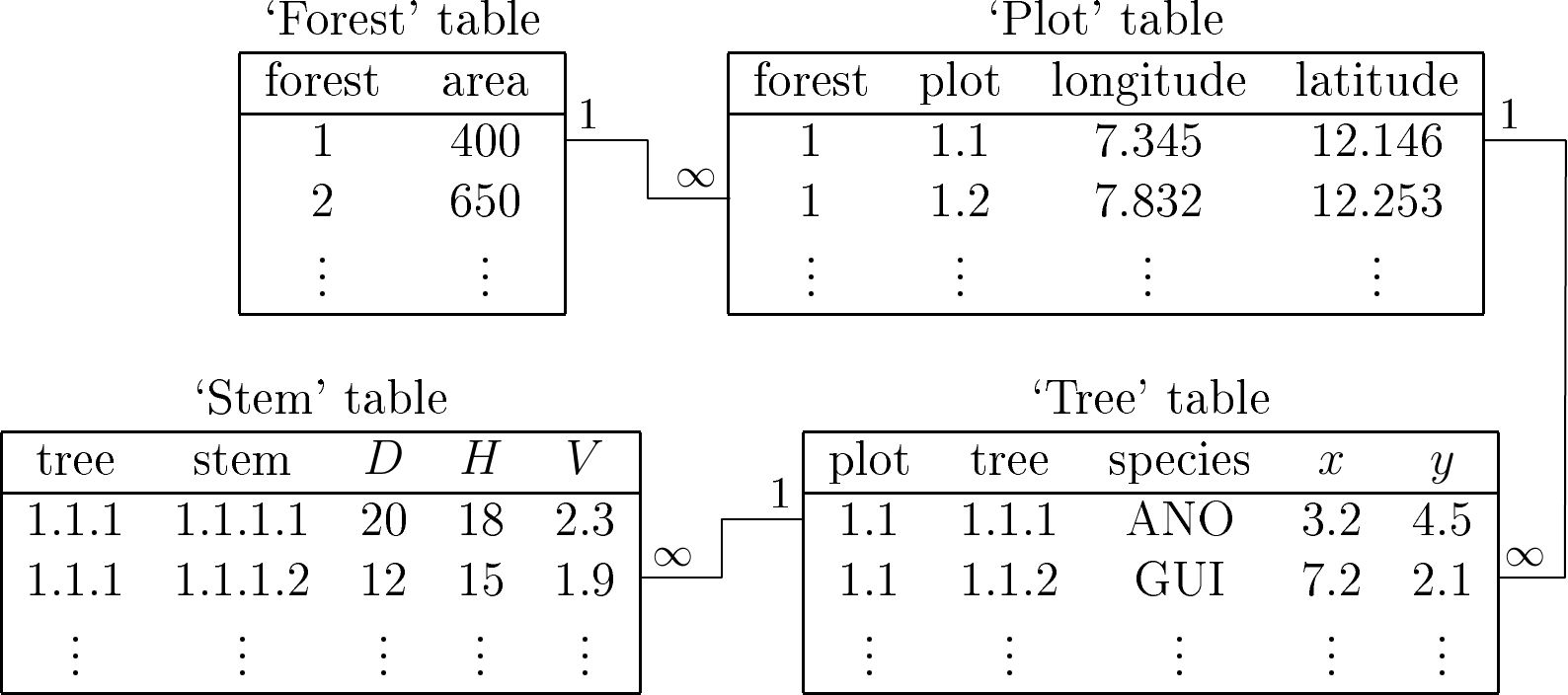
Figure 4.1: Example of four data tables for four nested levels.
| forest | area | plot | longitude | latitude | tree | species | \(x\) | \(y\) | stem | \(D\) | \(H\) | \(V\) |
|---|---|---|---|---|---|---|---|---|---|---|---|---|
| 1 | 400 | 1.1 | 7.345 | 12.146 | 1.1.1 | ANO | 3.2 | 4.5 | 1.1.1.1 | 20 | 18 | 2.3 |
| 1 | 40\(\textit{1}\) | 1.1 | 7.345 | 12.146 | 1.1.1 | ANO | 3.2 | 4.5 | 1.1.1.2 | 12 | 15 | 1.9 |
| 1 | 400 | 1.1 | 7.345 | 12.146 | 1.1.2 | GUI | 7.2 | 2.1 | \(\vdots\) | \(\vdots\) | \(\vdots\) | \(\vdots\) |
| 1 | 400 | 1.2 | 7.832 | 12.253 | \(\vdots\) | \(\vdots\) | \(\vdots\) | \(\vdots\) | \(\vdots\) | \(\vdots\) | \(\vdots\) | \(\vdots\) |
| 2 | 650 | \(\vdots\) | \(\vdots\) | \(\vdots\) | \(\vdots\) | \(\vdots\) | \(\vdots\) | \(\vdots\) | \(\vdots\) | \(\vdots\) | \(\vdots\) | \(\vdots\) |
| \(\vdots\) | \(\vdots\) | \(\vdots\) | \(\vdots\) | \(\vdots\) | \(\vdots\) | \(\vdots\) | \(\vdots\) | \(\vdots\) | \(\vdots\) | \(\vdots\) | \(\vdots\) | \(\vdots\) |
Giving the data this structure minimizes the amount of information entered, and therefore minimizes data entry errors. An alternative consists in entering all the data in a single data table, as indicated for instance in Table 4.1. This is not recommended as data is unnecessarily repeated and therefore the risk of making data entry errors is greatly increased. For instance, in Table 4.1 we have deliberately introduced a data entry error in the second line of the data table, where the area of forest 1, which should be 400 ha, here is 401 ha. By unnecessarily repeating the information, we find ourselves multiplying this type of inconsistency that must subsequently be corrected.
An effective method that can be used to resolve these nested level problems is to build a relational database. This type of database is specifically intended to manage different inter-related data tables. It removes all inconsistencies, such as that illustrated in Table 4.1 by systematically checking relational integrity between the tables. But building a relational database requires technical knowledge, and a person with skills in this field may need to be called upon.
In brief, when entering data, it is advisable to:
avoid repeating the same information,
prefer relational databases,
provide additional information (meta-information),
take great care with units,
distinguish between qualitative and quantitative information,
check the data,
reduce or correct missing data.
4.2 Data cleansing
Data cleansing requires toing-and-froing between the data record forms and the statistical software (or use of specially designed data cleansing software). This step aims to remove all data inconsistencies. And, if the measurement system is still in place, it may require certain measurements to be repeated. Data cleansing removes:
aberrant data. For example, a tree 50 meters in diameter.
inconsistent data. For example, a tree with a trunk biomass of 755 kg and a total biomass of 440 kg, or a tree that is 5 cm in diameter and 40 m in height.
false categories for qualitative variables. For example, software that differentiates between upper case and lower case will interpret “yes” and “Yes” as two different categories, whereas in fact they are the same.
The difficulty inherent to detecting aberrant data lies in choosing the threshold between what is a normal measurement and what is an aberrant measurement. It may happen that aberrant data stem from a change in unit during data entry. If the field data record form mentions 1.2 kg then 900 g for leaf biomass measurements, care must be taken to enter 1.2 and 0.9 (en kg), or 1200 and 900 (in g), not 1.2 and 900. Inconsistent data are more difficult to detect as they require the comparison of several variables one with another. In the example given above, it is perfectly normal for a tree to have a trunk biomass of 755 kg, as it is for a tree to have a total biomass of 440 kg, but obviously the two values cannot be simultaneously correct for the same tree. Likewise, there is nothing abnormal about a tree having a diameter of 5 cm, or a tree being 40 m high. It is simply that a tree with a diameter of 5 cm and a height of 40 m is abnormal.
Aberrant data and data inconsistencies can be detected using descriptive statistics and by plotting two variables one against the other: an examination of means, quantiles, and maximum and minimum values, will often detect aberrant data; plots of two variables one against the other can be used to detect inconsistent data. For instance, in the above example, we could plot total biomass against trunk biomass, and check that all the points are located above the line \(y=x\). Plots of height against diameter, volume against diameter, etc. can also be used to detect abnormal data. The categories describing qualitative variables could also be inspected by counting the number of observations per category. Two qualitative variables could then be crossed by building the corresponding contingency table. It should be assumed, during this inspection, that the statistical software has correctly interpreted numerical data as numerical data and qualitative data as qualitative data.
False categories often stem from sloppy data entry. Involuntary spelling mistakes are often made when entering the names of species in full, and this generates false categories. False categories may also be very ambiguous and difficult to correct. Let us consider the example of a dataset of trees in Central African wet tropical forest which, among other things, contains two species: alombi (Julbernardia seretii) and ilomba (Picnanthus angolensis). Let us assume that, by mistake, the false category “alomba” was entered. This false category differs from the true alombi and ilomba categories by only one letter. But which is the right category? Accents are also often the source of false categories, depending on whether text was entered with or without accents. Let us for example consider the entering of a color: for the person entering the data (in French) it may be perfectly clear that “vert foncé” and “vert fonce” are the same thing, but the software will consider these as two different categories. Masculines and feminines (again in French) may also pose a problem. “Feuille vert clair” and “feuille verte clair” will be understood by the software as two different categories. A false category often found is generated by a space. The “green” category (no space) and the “green␣” category (with a space, shown here by “␣”) will be understand by the software as two different categories. This false category is particularly difficult to detect as the space is invisible on the screen and the user therefore has the impression that the two categories are the same. All invisible characters (carriage return, tabulation, etc.) and characters that appear in the same fashion on the screen but have different ASCII codes, may generate the same type of confusing error.
False categories can be avoided by using data entry templates that restrict the entering of qualitative variable to a choice among admissible categories. Automatic data cleansing scripts, that remove incorrect spaces, check accents or letter upper or lower case, and check that qualitative variables take their value from a list of admissible categories, are a necessity for large datasets.
4.3 Data formatting
This formatting consists in organizing the data into a format suitable for the calculations needed to construct the model. Typically, this consists of a model with one line per statistical individual (a tree for an individual model, a plot for a stand table) and as many columns as there are descriptive variables (i.e. variables predicting biomass, volume…), and as there are effect variables (dbh, height…). This formatting phase may require advanced data handling techniques. In some cases the data will need to be aggregated from one descriptive level to another. For example, if we are looking to construct an individual model for a coppice, and the measurements were made on stems, the data concerning the stems of a given stump will need to be aggregated: add together the volumes and masses, and calculate the equivalent diameter (i.e. the quadratic mean) of the stump from the diameters of its stems. Another example is the construction of a stand model from measurements in individual trees. In this case the data regarding the trees need to be aggregated into data characterizing the stand (volume per hectare, dominant height, etc.). In the opposite case, datasets need to be split. For example, we have calculated the volume of trees selected at random in a multispecific stand, and we are looking to construct a separate model for the five dominant species: the dataset needs to be split on the basis of tree species.
This data formatting will be greatly facilitated if the data were initially entered in an appropriate format. In this matter, relational databases have the advantage of offering a search language that can be used to construct the appropriate tables easily. In Microsoft Excel, the notion of “pivot table” can also usefully be employed to format data.
- (@eq- counter: not full red / 1 to n / cross ref but no link and no list)
Red line 4.1 \(\looparrowright\) Red line dataset (hacking exercise environmment:not full red / section based number / cross ref and listing available)
To illustrate specific points in this guide we will be using a dataset collected in Ghana by Henry et al. (2010). This dataset gives the dry biomass of 42 trees belonging to 16 different species in a wet tropical forest. The diameter at breast height of each tree was measured, together with its height, the diameter of its crown, the mean density of its wood, its volume, and its dry biomass in five compartments: branches, leaves, trunk, buttresses, and total biomass.
Table 4.2 gives the data Henry et al. (2010) as they should be presented in a spreadsheet. The data table in the spreadsheet takes the form of a data rectangle; it should not contain any empty lines or empty columns, and its layout must not deviate from this matrix-like format. Decorative effects, indentations, cells left empty to “lighten” its appearance are to be avoided as the statistical software will be unable to read a dataset that deviates from a matrix format. Column headings should be reduced to short words, or even abbreviations. Information on the significance of these variables, and their units, should be presented separately in the meta-information.
If information needs to be entered about species, this should be entered in a second table as this involves two nested levels: the species level, with several trees per species, and the tree level nested in the species level. Thus, if we are looking to enter the ecological guild and the vernacular name of the species, this will generate a second Table 4.3 specific to the species where the scientific name of the species is used to create the link between Table 4.2 and Table 4.3.
Data reading.
Let us suppose that the data formatted in the matrix format have been saved in the Excel file
Henry_et_al2010.xls, the first worksheet of which, called biomass, contains Table 4.2. In R software, these data are read using the commands:
library(RODBC)
ch <- odbcConnectExcel("Henry_et_al2010.xls")
dat <- sqlFetch(ch, "biomass")
odbcClose(ch)
The data are then stored in the object dat.
Data cleansing.
A few checks may be performed to verify data quality. In R, the command summary generates basic descriptive statistics for the variables in a data table:
In particular for diameter at breast height, the result is:
##    Min. 1st Qu.  Median    Mean 3rd Qu.    Max.
##    2.60   15.03   59.25   58.59   89.75  180.00
Thus tree dbh varies from 2.6 cm to 180 cm, with a mean of 58.59 cm and a median of 59.25 cm. Basic descriptive statistics for total dry biomass Btot are as follows:
##    Min. 1st Qu.  Median    Mean 3rd Qu.    Max.
##  0.0000  0.1375  3.1500  6.8155  9.6075 70.2400
The total dry biomass of the largest tree is 70.24 tonnes. The dry biomass of the smallest tree in the dataset is zero. As biomass is expressed in tonnes to two decimal places, this zero value is not aberrant, it means simply that the dry biomass of this tree is less than 0.01 tonnes = 10 kg. This zero value will nevertheless pose a problem in the future when we want to log-transform the data.
Finally, we can check that the total dry biomass is indeed the sum of the biomasses of the four other compartments:
The greatest difference in absolute value is 0.01 tonnes, which indeed corresponds to the precision of the data (two significant figures). The dataset therefore does not contain any inconsistencies at this level.
| species | dbh | heig | houp | dens | volume | Bbran | Bfol | Btronc | Bctf | Btot |
|---|---|---|---|---|---|---|---|---|---|---|
| Heritiera utilis | 7.3 | 5.1 | 3.7 | 0.58 | 0.03 | 0.02 | 0.00 | 0.00 | 0.00 | 0.02 |
| Heritiera utilis | 12.4 | 12.0 | 5.0 | 0.62 | 0.11 | 0.02 | 0.00 | 0.05 | 0.00 | 0.07 |
| Heritiera utilis | 31.0 | 22.0 | 9.0 | 0.61 | 1.34 | 0.10 | 0.01 | 0.71 | 0.02 | 0.83 |
| Heritiera utilis | 32.5 | 27.5 | 7.1 | 0.61 | 1.12 | 0.07 | 0.01 | 0.61 | 0.01 | 0.70 |
| Heritiera utilis | 48.1 | 35.6 | 7.9 | 0.61 | 3.83 | 0.24 | 0.01 | 2.07 | 0.01 | 2.33 |
| Heritiera utilis | 56.5 | 35.1 | 8.0 | 0.60 | 5.43 | 0.85 | 0.03 | 2.28 | 0.14 | 3.31 |
| Heritiera utilis | 62.0 | 40.4 | 11.1 | 0.60 | 6.84 | 0.68 | 0.04 | 3.28 | 0.15 | 4.15 |
| Heritiera utilis | 71.9 | 42.3 | 20.0 | 0.60 | 9.84 | 1.34 | 0.05 | 4.43 | 0.11 | 5.93 |
| Heritiera utilis | 83.0 | 39.4 | 15.9 | 0.60 | 11.89 | 2.20 | 0.09 | 4.83 | 0.04 | 7.16 |
| Heritiera utilis | 100.0 | 50.5 | 19.1 | 0.58 | 31.71 | 8.71 | 0.11 | 8.39 | 1.40 | 18.61 |
| Heritiera utilis | 105.0 | 50.5 | 19.2 | 0.58 | 35.36 | 8.81 | 0.13 | 11.18 | 0.65 | 20.76 |
| Heritiera utilis | 6.5 | 8.1 | 1.5 | 0.78 | 0.01 | 0.01 | 0.00 | 0.00 | 0.00 | 0.01 |
| Tieghemella heckelii | 12.0 | 17.0 | 4.7 | 0.78 | 0.15 | 0.12 | 0.01 | 0.00 | 0.00 | 0.13 |
| Tieghemella heckelii | 73.5 | 45.0 | 11.1 | 0.66 | 11.08 | 1.27 | 0.04 | 5.91 | 0.14 | 7.36 |
| Tieghemella heckelii | 80.5 | 50.7 | 13.0 | 0.66 | 12.25 | 1.54 | 0.05 | 6.45 | 0.09 | 8.13 |
| Tieghemella heckelii | 93.0 | 45.0 | 17.0 | 0.66 | 17.79 | 3.66 | 0.06 | 7.80 | 0.21 | 11.73 |
| Tieghemella heckelii | 180.0 | 61.0 | 41.0 | 0.62 | 112.81 | 27.28 | 0.74 | 35.07 | 7.16 | 70.24 |
| Piptadeniastrum africanum | 70.0 | 39.7 | 10.5 | 0.58 | 10.98 | 2.97 | 0.06 | 3.29 | 0.07 | 6.39 |
| Piptadeniastrum africanum | 89.0 | 50.0 | 18.8 | 0.57 | 15.72 | 3.69 | 0.05 | 5.16 | 0.16 | 9.06 |
| Piptadeniastrum africanum | 90.0 | 50.2 | 16.0 | 0.57 | 22.34 | 5.73 | 0.38 | 6.23 | 0.74 | 13.08 |
| Aubrevillea kerstingii | 65.0 | 32.5 | 9.0 | 0.62 | 4.79 | 1.52 | 0.02 | 1.45 | 0.00 | 2.99 |
| Afzelia bella | 83.6 | 40.0 | 13.5 | 0.67 | 14.57 | 3.17 | 0.03 | 6.00 | 0.58 | 9.79 |
| Cecropia peltata | 7.8 | 2.3 | 2.5 | 0.17 | 0.07 | 0.00 | 0.00 | 0.01 | 0.00 | 0.01 |
| Cecropia peltata | 20.5 | 21.2 | 6.2 | 0.23 | 0.44 | 0.03 | 0.00 | 0.07 | 0.00 | 0.11 |
| Cecropia peltata | 29.3 | 22.5 | 8.9 | 0.27 | 1.11 | 0.13 | 0.01 | 0.16 | 0.00 | 0.31 |
| Cecropia peltata | 35.5 | 12.0 | 7.3 | 0.26 | 1.39 | 0.12 | 0.02 | 0.25 | 0.00 | 0.38 |
| Ceiba pentandra | 132.0 | 45.0 | 16.0 | 0.54 | 28.55 | 1.53 | 0.04 | 13.37 | 0.44 | 15.39 |
| Ceiba pentandra | 170.0 | 51.0 | 27.1 | 0.26 | 64.84 | 3.20 | 0.10 | 11.87 | 1.88 | 17.05 |
| Nauclea diderrichii | 2.6 | 4.9 | 8.4 | 0.76 | 0.00 | 0.00 | 0.00 | 0.00 | 0.00 | 0.00 |
| Nauclea diderrichii | 94.6 | 50.5 | 12.0 | 0.50 | 17.19 | 1.06 | 0.02 | 7.49 | 0.06 | 8.64 |
| Nauclea diderrichii | 110.0 | 58.8 | 14.1 | 0.40 | 28.71 | 3.47 | 0.06 | 7.90 | 0.07 | 11.49 |
| Nauclea diderrichii | 112.0 | 40.0 | 13.2 | 0.47 | 22.74 | 3.41 | 0.10 | 7.19 | 0.13 | 10.82 |
| Daniellia thurifera | 9.0 | 9.3 | 8.0 | 0.42 | 0.11 | 0.05 | 0.01 | 0.00 | 0.00 | 0.05 |
| Guarea cedrata | 12.8 | 13.0 | 3.1 | 0.62 | 0.12 | 0.08 | 0.01 | 0.00 | 0.00 | 0.08 |
| Guarea cedrata | 71.5 | 45.5 | 14.0 | 0.50 | 10.12 | 0.65 | 0.02 | 4.30 | 0.13 | 5.10 |
| Strombosia glaucescens | 7.6 | 11.3 | 3.9 | 0.66 | 0.07 | 0.05 | 0.01 | 0.00 | 0.00 | 0.05 |
| Strombosia glaucescens | 26.5 | 26.0 | 12.2 | 0.73 | 1.09 | 0.20 | 0.01 | 0.58 | 0.00 | 0.80 |
| Garcinia epunctata | 7.1 | 5.7 | 3.8 | 0.65 | 0.08 | 0.05 | 0.01 | 0.00 | 0.00 | 0.06 |
| Drypetes chevalieri | 13.2 | 15.7 | 5.0 | 0.65 | 0.22 | 0.15 | 0.02 | 0.00 | 0.00 | 0.16 |
| Cola nitida | 23.6 | 23.4 | 6.3 | 0.56 | 0.68 | 0.09 | 0.01 | 0.28 | 0.00 | 0.39 |
| Nesogordonia papaverifera | 24.3 | 30.2 | 6.5 | 0.69 | 0.73 | 0.12 | 0.01 | 0.36 | 0.02 | 0.51 |
| Dialium aubrevilliei | 98.0 | 43.7 | 98.0 | 0.65 | 18.49 | 2.55 | 0.05 | 9.07 | 0.40 | 12.07 |
| guild | species | vernacular |
|---|---|---|
| non-pioneer light demanding | Heritiera utilis | Nyankom |
| non-pioneer light demanding | Tieghemella heckelii | Makore |
| non-pioneer light demanding | Piptadeniastrum africanum | Dahoma |
| non-pioneer light demanding | Aubrevillea kerstingii | Dahomanua |
| non-pioneer light demanding | Afzelia bella | Papao-nua |
| pioneer | Cecropia peltata | Odwuma |
| pioneer | Ceiba pentandra | Onyina |
| pioneer | Nauclea diderrichii | Kusia |
| pioneer | Daniellia thurifera | Sopi |
| shade bearer | Guarea cedrata | Kwabohoro |
| shade bearer | Strombosia glaucescens | Afena |
| shade bearer | Garcinia epunctata | Nsokonua |
| shade bearer | Drypetes chevalieri | Katreka |
| shade bearer | Cola nitida | Bese |
| shade bearer | Nesogordonia papaverifera | Danta |
| shade bearer | Dialium aubrevilliei | Dua bankye |