3 In the field
The field step is the most crucial as it may generate measurement errors that cannot be corrected. This phase must be governed by three key principles: (i) it is better to weigh everything in the field rather than calculate a volume and multiply it later by a density measurement (see chapter 1 and variations in stem shape and wood density); (ii) if wood aliquots are taken, it is best to weigh the whole then the aliquot to follow moisture loss; finally (iii) as a biomass campaign requires a great deal of work and is very costly to undertake, other measurements may be taken at the same time to avoid a subsequent return to the field (e.g. stem profile, sampling for nutrient content).
Selecting trees to be measured in the field (see chapter 2), whether as individuals or exhaustively over a given area, means that the trees must be marked with paint, measured for circumference if possible at breast height (by circling the trunk with paint at this point) and measured for height. This procedure is used to check that the tree selected indeed corresponds to the sampling plan chosen (case of a selection by individual) and provides for control measures once the tree has been felled. It is also very practical to take a photo of the individual selected and draw a schematic diagram of the tree on the field form. This makes it easier to interpret the data and check the results obtained. In general, trees that are too unusual (crown broken, stem knotty or sinuous) should not be selected unless these stems account for a significant proportion of the stand, or if the aim is to quantify an accident (e.g. crown breaking subsequent to frost). Likewise, trees located in an unrepresentative environment should be excluded (forest edge, clearing, degraded forest, etc.) as their architecture often differs from the other trees in the stand. Finally, field constraints (slope, access, stand non compliant with the stratum, etc.) may well call the original sampling into question.
The general basis for measuring biomass, and even more nutrient content, is the rule of three between fresh biomass measured in the field, fresh biomass of the aliquot, and oven-dried biomass of the aliquot. As the different organs of a tree do not have the same moisture content or the same density, it is preferable to proceed by compartmentalization to take account of variations in tree density and moisture content (and nutrient concentrations when calculating nutrient content). The finer the stratification, the more precise the biomass estimation, but this requires a great deal more work. A compromise must therefore be found between measurement precision and work rate in the field. Conventionally, a tree is divided into the following compartments: the trunk, distinguishing the wood from the bark, and that should be sawed into logs to determine variations in density and moisture content in relation to section diameter; branches that are generally sampled by diameter class, distinguishing or not the wood from the bark; the smallest twigs, generally including buds; leaves; fruits; flowers; and finally roots by diameter class. An example of a such a compartmentalization is given in Figure 3.1 for beech.

Figure 3.1: Example of tree compartmentalization for a biomass and nutrient content campaign on beech in France.
Full advantage may be made of existing felling operations to sample the trees necessary to establish the table, particularly given that access and the taking of samples is often regulated in forests, and silviculture provides one of the only means to access the trees sought. However, this method may induce bias in tree selection as mainly commercial species are felled. Other species are felled only if they hinder the removal of a tree selected by the timber company, or if they are located on conveyance tracks or in storage areas. Also, trees felled for commercial purposes cannot necessarily be cross-cut into logs of a reasonable size to be weighed in the field. This depends on the capacity of the weighing machines available and log length. These constraints mean that individuals need to be carefully selected and two methods combined: (1) all the non-commercial sections of the tree must be weighed, particularly the branches; (2) the volume and wood density of the trunk must be determined.
Therefore, in the field, there is no standard method as operators must adapt to each situation. But, here in this guide, we will nevertheless describe three typical cases that can be employed subsequently as the basis for conducting any type of field campaign. The first concerns regular forest (derived from regeneration or planted), the second dry forest and the third wet tropical forest. In the first case, all the compartments are weighed directly in the field. In the second, as the trees cannot be felled, the measurements made are semi-destructive. The third case concerns trees that are too large to be weighed in their entirety in the field. Measurements are therefore obtained in three phases: in the field, in the laboratory, then by computation. As the field measurements and computations are specific to each method, they are presented for each individual case. The laboratory procedures are generally the same in all cases.
3.1 Weighing all compartments directly in the field
The first case we will tackle is the most common and involves directly weighing all the compartments in the field. The operating procedure suggested is the fruit of several field campaigns conducted both in temperate and tropical climates. We will illustrate the case by examples taken from a variety of regular stands: plantations of eucalyptus in Congo (Saint-André et al. 2005), rubber tree in Thailand, and high forests of beech and oak in France (Genet et al. 2011). An example of this methodology, with additional measurements on the tapering of large branches, and sampling for nutrient content, is given by Rivoire et al. (2009).
3.1.1 In the field
Logging is a complex business and must be smoothly organized such that all the various teams are always working, with no slack periods (see 3.6 for details on these teams). It must be prepared in advance by the logging manager who preselects the trees and marks them in the forest. This is followed by laboratory work to (i) prepare the necessary materials (see 3.5 for details), (ii) prepare data record forms (weights of the different compartments, connected measurements), (iii) prepare bags to receive the aliquots taken from the trees (see 3.1), (iv) explain to the different operators how logging is organized so that all know what to do in the field. Figure 3.2 illustrates an effective organization for a biomass campaign, with seven operations being undertaken at the same time.
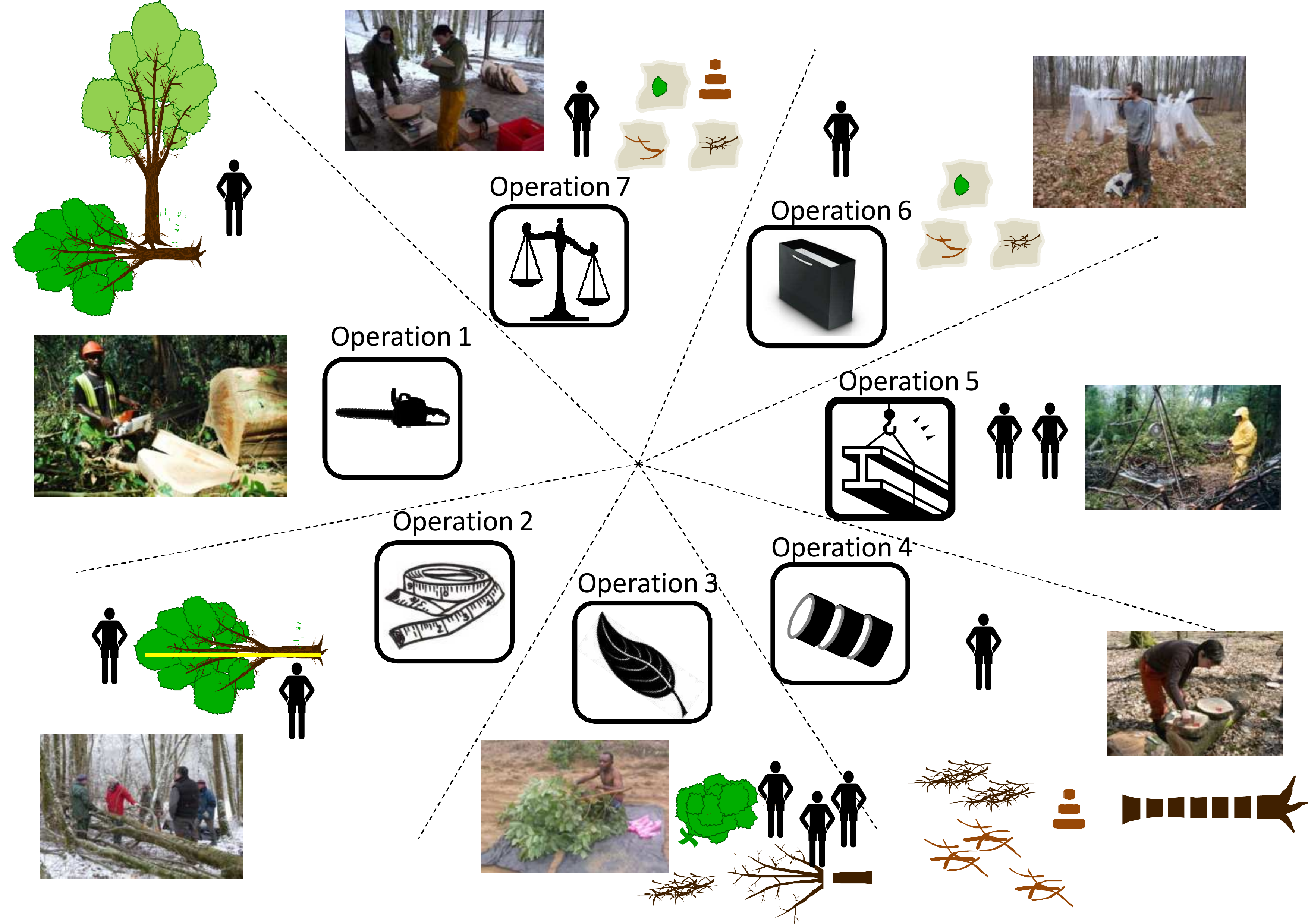
Figure 3.2: Organization of a biomass measurement site with 7 different operations. Operation 1, site preparation and felling of the trees (photo: L. Saint-André); operation 2, measurement of felled trees: stem profile, marking for cross-cutting (photo: M. Rivoire); operation 3, stripping of leaves and limbing (photo: R. D’Annunzio and M. Rivoire); operation 4, cross-cutting into logs and disks (photo: C. Nys); operation 5, weighing of logs and brushwood (photo: J.-F. Picard); operation 6, sampling of branches (photo: M. Rivoire); operation 7, sample weighing area (photo: M. Rivoire).
Given that limbing time is the longest, it may be useful to start with a large tree (photo 3.3). The site manager accompanies the loggers and places the sample bags at the base of the tree (operation 1). Bag size must be suitable for the size of the sample to be taken. The bags must systematically be labeled with information on compartment, tree and plot. After felling, the first team to intervene is that which measures stem profile (operation 2). Once this team has finished, it moves on to the second tree that the loggers have felled in the meantime while the limbing teams start work on the first tree (operation 3). A 12-tonne tree (about 90–100 cm in diameter) takes about half a day to process in this way. By the time limbing has been completed on the first tree, the loggers have had time to fell sufficient trees in advance to keep the profiles team busy for the rest of the day. The loggers can now return to the first tree for cross-cutting into logs, and to cut disks (operation 4). Once the cross-cutting and disk cutting has been completed on the first tree, the loggers can move on to the second tree that in the meantime has been limbed. The leaves, logs and branches from the first tree can now be weighed (operation 5) while the site manager takes samples of leaves and branches (operation 6). All the samples, including the disks, must be carried to the sample weighing area (operation 7). Once the stem profiling team has finished all the trees for the day, it can come to this area to complete the weighing operations.
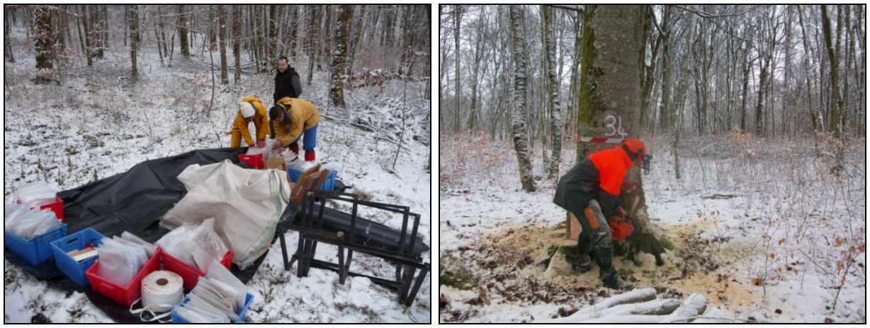
Figure 3.3: Measurement campaign in a high forest coppice in France. On the left, arriving at the site and deploying equipment (photo: M. Rivoire); on the right, felling the first tree (photo: L. Saint-André).
This chronological process is valid under temperate climatic conditions. In the tropics, it is impossible to wait for the end of the day before weighing the samples. The samples taken must therefore be weighed at the same time as the logs and brushwood. If the samples cannot be weighed in situ, they must be weighed in the laboratory, but in this case they must be shipped in a tightly sealed box to reduce evaporation of the water they contain. This should be considered as a last resort since weighing in the field is more reliable.
Felling (operation 1)
The logger prepares the tree selected while the technicians cut any small stems that may hinder the tree’s fall and clear the area. A tarpaulin may be spread on the ground so as not to lose any leaves when felling (photo 3.4). As the tree’s fall may bring down branches from other crowns, the technicians separate these from those of the selected tree.

Figure 3.4: Biomass campaign in a eucalyptus plantation in Congo. On the left, stripping leaves onto a tarpaulin (photo: R. D’Annunzio). On the right, operations completed for a tree, with bags in the weighing area containing leaves, logs and brushwood (photo: L. Saint-André).
Measuring the tree (operation 2)
Stem profiles are then measured (photo 3.5). As the trunk is never cut at ground level, it is vital to mark the tree at breast height (1.30 m) with paint prior to felling, and place the measuring tape’s 1.30 m graduation on this mark once the tree has been felled. This avoids any introduction of bias in section location (the shift induced by cutting height). Circumferences are generally measured every meter or, more usefully for constructing stem profile models, by percentage of total height. This latter method, however, is far more difficult to apply in the field. If it is impossible to measure a circumference because the trunk is flat on the ground, use tree calipers to take two diameter measurements, one perpendicular to the other. When moving up the trunk, the cross-cutting points agreed with the forest management organization (or timber buyer) should be marked on the trunk with paint or a logger’s mark.
If the tree is straight and has a clearly identified main stem, there is no need to choose a principal axis. But if the stem is very twisted or branched (crown of hardwoods), the principal axis needs to be identified. This should then be marked, for instance with paint. The principal axis differs from the others by having the largest diameter at each fork in the trunk. All branched axes on the main stem are considered to be branches. It is possible, in the case of multistemmed trees, either to include each stem in the principal stem (photo 3.6), or consider each stem as an individual and in this case trace the principal axis on each.
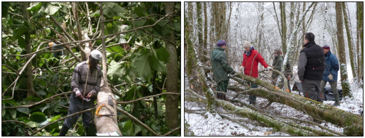
Figure 3.5: Left, biomass campaign in Ghana in a teak high forest: measurement of branching (photo: S. Adu-Bredu). Right, biomass campaign in France in a high forest coppice: stem profile measurements (photo: M. Rivoire).
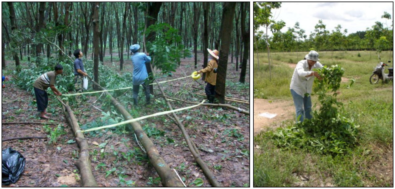
Figure 3.6: Biomass campaign in rubber tree plantations in Thailand. Left, a multistemmed felled tree (3 stems on the same stump): limbing and stripping of the leaves. Right, leaves mixed together prior to aliquoting (photos: L. Saint-André).
The length of the trunk and the position of the last live branch and major forks must then be determined. Various heights can be measured on the felled tree, for example: height at the small end \(<1\) cm, height at cross-cut diameter 4 cm, and height at cross-cut diameter 7 cm. The measurements made on the felled tree can then be compared with those made in standing trees during forest inventories. This checks dataset consistency and can be used to correct aberrant data, though differences may of course arise from the imprecision of pre-felling height measurements (generally 1 m), or from stem sinuosity or breakages when measuring post-felling lengths.
Cross-cutting (operations 3 and 4)
Ideally, the tree should be cut into 2 m logs to take account of wood density and moisture content variations in the stem. Once the tree has been prepared, the branches (and if necessary the leaves) must be separated from the trunk. The branches should then be cut to prepare bundles by small end class. When dealing with a stand of temperate hardwoods, the stem is generally cut into diameter classes of \(>20\) cm, 20–7 cm, 7–4 cm, \(<4\) cm. For eucalyptus in the DR of Congo, the branches were split into two groups: \(<2\) cm and \(>2\) cm. Branch bundles were prepared on an iron frame with two pieces of strong string (see 3.5 and photo 3.20). If the branches bear leaves, these leaves should be stripped off the twigs. Tarpaulins should be used in this case to avoid losing any leaves. If the leaves are difficult to remove from the woody axes (e.g. holm oak or softwoods), a subsampling strategy should be adopted (see the example below for Cameroon). The leaves are placed in large plastic bags for weighing. Limbing and leaf stripping take time, and sufficient human resources (number of teams) should be allocated so as not to slow the loggers in their work. The limbs of the tree are often large in diameter (\(>20\) cm) and should be processed in the same manner as for the trunk, by cross-cutting into logs and disks.
This cross-cutting should take place once the limbs have been separated from the main trunk. A disk about 3–5 cm thick should be taken from the stump, then every \(x\) meters (photo 3.7). Log length \(x\) depends on the dimensions of the tree and the agreements established with the body in charge of the forest or the timber company. As this field work is tedious and time-consuming, full advantage should be made of this time spent in the field to take multiple samples (e.g. an extra disk for more detailed measurements of wood density or nutrient content — see for instance Saint-André, Laclau, Deleporte, et al. 2002, for nutrient concentrations in the stems of eucalyptus). It is important to indicate the position of each disk taken. These disks must be weighed in situ on the day the tree was processed to reduce moisture losses (this operation requires work by two people — generally the stem profiling team performs this task by taking a break from its work a little earlier to weigh the disks, see 3.2).
Weighing logs and brushwood bundles (operation 5)
The logs and bundles produced are weighed in the field (photo 3.7) and within a short timeframe to ensure that the measurements for a given tree were taken under the same relative humidity conditions. The most practical approach here is to use hanging scales attached to a digger. The bundles are attached to the scales and fresh weight measured. The string and the tarpaulin can then be recovered for reuse.

Figure 3.7: Biomass campaign in an oak grove. Left, disks taken and placed in large bags for transfer to the samples weighing area; middle, samples weighing area; right, digger used to weigh logs (photos: C. Nys).
Taking aliquots (operations 6 and 7)
Once the bundles have been weighed, aliquots are taken from each to estimate branch moisture content. Samples of different diameters should be taken from different branches to be representative of the architecture of a standard branch: sampling a single branch could lead to bias if it is more wet or dry than the others. The branches should be split into four diameter groups (class 1: \(0<\varnothing\leq4\) cm, class 2: \(4<\varnothing\leq7\) cm, class 3: \(7<\varnothing\leq20\) cm, and class 4: \(\varnothing>20\) cm). Samples about 10 cm long should be taken of the class 1 branches. A similar principle applies for the other branches, but as they are larger in diameter, disks are taken instead of pieces 10 cm long. About 9, 6 and 3 disks should be taken for classes 2, 3 and 4, respectively. These figures are only a rough guide but are nevertheless derived from a number of different campaigns conducted in different ecosystems. These aliquots are then placed in specially prepared paper bags (previously placed at the foot of the tree, see the first step). These paper bags are then placed in a plastic bag for a given tree to ensure that there is no mix up of samples between trees.
To avoid sampling bias, the same person must take all the samples and work in a systematic manner that is representative of the variability in each branch size class. To minimize bias when measuring moisture content, all the samples should be taken to the weighing area (same place as the disks) and should be weighed in their paper bag before being processed in the laboratory. Although it is best to weigh the samples in the field, if this proves impossible then any loss of moisture should be avoided. For instance the use of a cool box is very highly recommended. When sampling leaves, they should first be mixed together and the sample should be taken randomly from the middle of the heap. This mixing-sampling operation should be conducted five or six times for each tree (photo 3.6). The samples from each tree should then be placed in the same bag (the amount taken should be adapted to leaf size and heterogeneity, and particularly the proportion of green to senescent leaves — one standard plastic bag is generally perfectly adequate).
3.1.2 In the laboratory
If the trunk disks cannot be measured immediately they should be stocked in the fresh air on wooden battens so that air can circulate freely between them (to avoid mould). They can now be left to dry provided that fresh biomass was measured in the field. But if they were not weighed in the field, they must be weighed immediately on arrival.
For aliquots that were weighed in a bag in the field, the weight of the empty bag must now be determined (if possible measure each bag, or if very damaged, weigh 10 to 20 bags and calculate mean weight). This value should then be deducted from the field measurements. If a fresh bag is used when drying the aliquots, this must bear all the necessary information.
The oven should be set at 70\(^{\circ}\)C for leaves, flowers and fruits, or at 65\(^{\circ}\)C if the aliquots are subsequently to undergo chemical analysis. A temperature of 105\(^{\circ}\)C should be used for biomass determinations, and only for wood. At least three controls should be weighed every day for all sample categories until a constant weight is reached. This avoids withdrawing actual samples from the oven for daily controls. Leaf weight generally stabilizes after two days, and woody structures after about one week depending on the size of the sample.
Figure 3.8 shows the operating procedure to be adopted for measuring the samples taken. Laboratory measurements begin by weighing the wet samples with their bag (measurement checking that made in the field). If the disks are too large, they may be subsampled. In this case it is vital to weight the full disk again, then the sample taken. Moisture lost from the disk between the field and the laboratory should be added to this laboratory measurement after drying the disk sample in the oven. If a great deal of time has elapsed between the field phase and the laboratory phase, and if this step in the protocol is overlooked, this may cause very considerable errors of up to 60 or 70% in dry biomass estimations. The bark is generally removed using a bark knife or a wood chisel (photo 3.9 — placing the disks in a freezer when still wet may facilitate this operation (e.g. for oak). Samples of the bark and wood are then measured and dried in the oven (take care not to place too many bags at once in the oven).
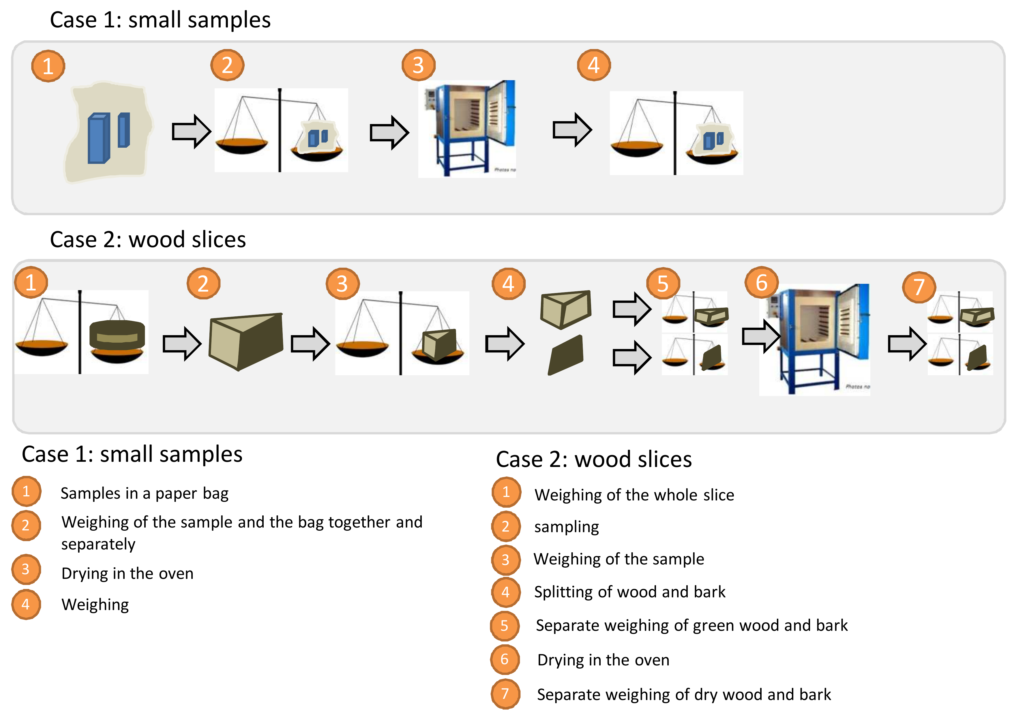
Figure 3.8: Weighing procedure for samples on arrival at the laboratory.
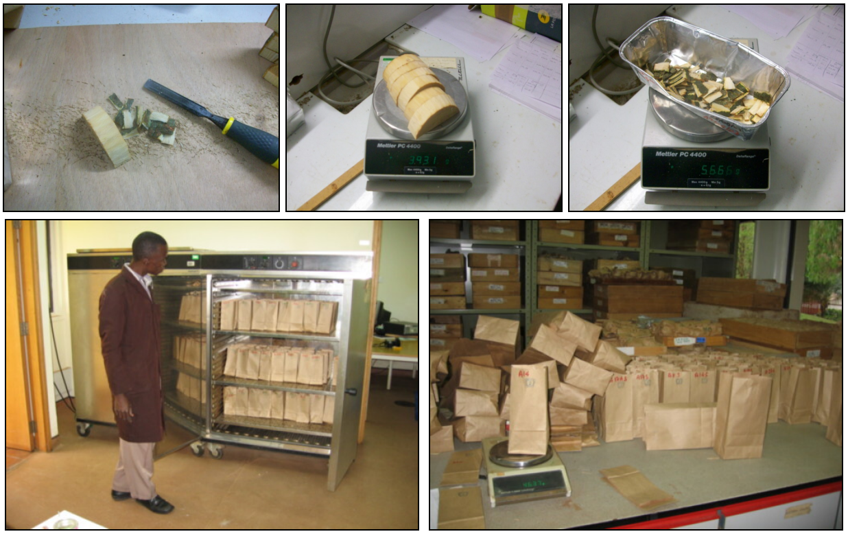
Figure 3.9: Laboratory measurements: (A) debarking, (B) weighing the wood, (C) weighing the bark (photos: L. Saint-Andr�), (D) oven-drying samples, (E) regular weighing to constant weight (photos: M. Henry).
3.1.3 Calculations
Calculating the biomass of the trunk
For each log \(i\), measure the circumference at the two extremities: circumference \(C_{1i}\) at the small end is the circumference of the disk taken at the small end and circumference \(C_{2i}\) at the large end is the circumference of the disk taken at the large end. This can be employed to calculate the volume of the fresh log using the truncated cone volume formula (or Newton’s formula): \[\begin{equation} V_{\text{fresh},i}=L_i\times\frac{\pi}{3}\times(R_{1i}^2+R_{1i}R_{2i} +R_{2i}^2)\tag{3.1} \end{equation}\] where \(L_i\) is the length of log \(i\), and \(R_{1i}=C_{1i}/(2\pi)\) and \(R_{2i}=C_{2i}/(2\pi)\) are the radii of log \(i\) at its two extremities. This volume may be measured with bark (circumferences being measured in the field) or without bark (circumferences being measured on the disks after debarking in the laboratory). Fresh volume with bark is widely employed when selling timber whereas the second measurement is used to check data consistency for it is used to calculate wood density in the tree.
It should be noted that other formulas are also used to calculate the volume of a log. That most commonly used is Huber’s formula (based on circumference measured in the middle of the log) and Smalian’s formula (based on the quadratic mean of the circumferences measured at the top and bottom of the log). But if the logs are short (1 or 2 m), their shape is little different from that of a cone, with very little tapering, and the difference between the formulas is very slight.
Also, for each sample taken of log \(i\) we calculate:
the proportion of fresh biomass in the wood (without the bark): \[ \omega_{\text{fresh wood},i}=\frac{B^{\text{aliquot}}_{\text{frresh wood},i}}{B^{\text{aliquot}}_{\text{fresh wood},i}+B^{\text{aliquot}}_{\text{fresh bark},i}} \] where \(B^{\text{aliquot}}_{\text{fresh wood},i}\) is the fresh biomass of the wood (without the bark) in the sample of log \(i\), and \(B^{\text{aliquot}}_{\text{fresh bark},i}\) is the fresh biomass of the bark in the sample of log \(i\);
the moisture content of the wood (without the bark): \[\begin{equation} \chi_{\text{wood},i}=\frac{B^{\text{aliquot}}_{\text{dry wood},i}}{B^{\text{aliquot}}_{\text{fresh wood},i}}\tag{3.2} \end{equation}\] where \(B^{\text{aliquot}}_{\text{dry wood},i}\) is the oven-dried biomass of the wood (without the bark) in the sample of log \(i\);
the proportion of fresh biomass in the bark: \[ \omega_{\text{fresh bark},i}=1-\omega_{\text{fresh wood},i} \]
the moisture content of the bark: \[ \chi_{\text{bark},i}=\frac{B^{\text{aliquot}}_{\text{dry bark},i}}{B^{\text{aliquot}}_{\text{fresh bark},i}} \] where \(B^{\text{aliquot}}_{\text{dry bark},i}\) is the oven-dried biomass of the bark in the sample of log \(i\).
We then extrapolate the values obtained for the sample of log \(i\) to the whole of log \(i\) by rules of three:
the oven-dried biomass of the wood (without the bark) in log \(i\) is: \[ B_{\text{dry wood},i}=B_{\text{fresh},i}\times \omega_{\text{fresh wood},i}\times\chi_{\text{wood},i} \] where \(B_{\text{fresh},i}\) is the fresh biomass (including the bark) of log \(i\);
the oven-dried biomass of the bark in log \(i\) is: \[ B_{\text{dry bark},i}=B_{\text{fresh},i}\times \omega_{\text{fresh bark},i}\times\chi_{\text{bark},i} \]
the density of the wood in log \(i\) is: \[ \rho_i=\frac{B_{\text{dry wood},i}}{V_{\text{fresh},i}} \] where \(V_{\text{fresh},i}\) is the fresh volume (without the bark) given by equation (3.1).
The weights of all the logs should then be summed to obtain the dry weight of the trunk:
the dry biomass of the wood (without the bark) in the trunk is: \[ B_{\text{trunk dry wood}}=\sum_iB_{\text{dry wood},i} \] where the sum concerns all logs \(i\) that make up the trunk;
the dry biomass of the bark in the trunk is: \[ B_{\text{trunk dry bark}}=\sum_iB_{\text{dry bark},i} \]
The wood density \(\rho_i\) used in the calculation of dry biomass must be the oven-dry wood density, i.e. the ratio of dry biomass (dried in the oven to constant dry weight) to the volume of fresh wood. Care should be taken not to confuse this wood density value with that calculated using the same moisture content for the mass and the volume (i.e. dry mass over dry volume or fresh mass over fresh volume). The AFNOR (1985) standard, however, defines wood density differently, as the ratio of the biomass of the wood dried in the fresh air to the volume of the wood containing 12 % water (Fournier-Djimbi 1998). But the oven-dry wood density can be calculated from the density of wood containing 12 % water using the expression (Gourlet-Fleury et al. 2011): \[ \rho_{\chi}=\frac{\rho\ (1+\chi)}{1-\eta\ (\chi_0-\chi)} \] where \(\rho_{\chi}\) is the ratio of the biomass of the wood dried in the fresh air to the volume of the wood containing \(\chi\) % water (in g cm-3), \(\rho\) is the ratio of the oven-dry wood density to the fresh volume of the wood (in g cm-3), \(\eta\) is the volumetric shrinkage coefficient (figure without dimensions) and \(\chi_0\) is the fibers saturation point. The coefficients \(\eta\) and \(\chi_0\) vary from one species to another and require information on the technological properties of the species’ wood. Also, using findings for \(\rho\) and \(\rho_{12\%}\) in 379 trees, Reyes et al. (1992) established an empirical relationship between oven-dry density \(\rho\) and density with 12 % water \(\rho_{12\%}\): \(\rho=0.0134+0.800\rho_{12\%}\) with a determination coefficient of \(R^2=0.988\).
Calculating the biomass of the leaves
For each sample \(i\) of leaves taken, calculate the moisture content: \[ \chi_{\text{leaf},i}=\frac{B^{\text{aliquot}}_{\text{dry leaf},i}}{B^{\text{aliquot}}_{\text{fresh leaf},i}} \] where \(B^{\text{aliquot}}_{\text{dry leaf},i}\) is the oven-dry biomass of the leaves in sample \(i\), and \(B^{\text{aliquot}}_{\text{fresh leaf},i}\) is the fresh biomass of the leaves in sample \(i\). We then, by a rule of three, extrapolate sample \(i\) to compartment \(i\) from which this sample was drawn: \[ B_{\text{dry leaf},i}=B_{\text{fresh leaf},i}\times \chi_{\text{leaf},i} \] where \(B_{\text{dry leaf},i}\) is the (calculated) dry biomass of the leaves in compartment \(i\), and \(B_{\text{fresh leaf},i}\) is the (measured) fresh biomass of the leaves in compartment \(i\). Often the entire crown corresponds to a single compartment. But if the crown has been compartmentalized (e.g. by successive tiers), the total dry weight of the leaves is obtained by adding together all compartments \(i\): \[ B_{\text{dry leaf}}=\sum_i B_{\text{dry leaf},i} \]
Calculating the biomass of the branches
If the branches are very large (e.g. \(>20\) cm in diameter), proceed as for the trunk, and for the brushwood proceed as for the leaves.
Calculating the biomass of fruits, flowers
The method is identical to that used for the leaves.
3.2 Direct weighing for certain compartments and volume and density measurements for others
The second case we consider here is that where felling constraints mean that only semi-destructive measurements are taken. These combine direct measurements for certain parts of the tree, and volume and density measurements for the others. We will illustrate this by developing an allometric equation for the dry northern forests of Cameroon. The biomass of dry forests is particularly difficult to determine given the architectural complexity of the trees they contain. Human intervention is also particularly significant in dry areas because of the rarity of forest resources and the magnitude of the demand for bioenergy. This is reflected by the trimming, pruning and maintenance practices often employed for trees located in deciduous forests, agro-forest parks and hedges (photo 3.10).
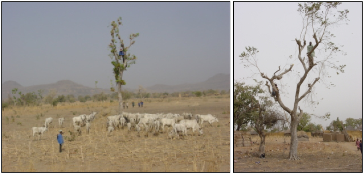
Figure 3.10: Trimming shea trees (Vitellaria paradoxa) in north Cameroon (photo: R. Peltier).
The trees in most dry areas are protected as this woody resource regenerates particularly slowly and is endangered by human activities. Biomass measurements are therefore non-destructive and take full advantage of this trimming to measure the biomass of the trimmed compartments. Grazing activities limit regeneration and small trees are often few in number. This part of the guide will therefore consider only mature trees.
3.2.1 In the field: case of semi-destructive measurements
Generally, the trunk and the large branches are not trimmed; only the small branches are affected. The measurement of fresh biomass (in kg) may be divided into two parts: measuring trimmed fresh biomass and measuring untrimmed fresh biomass (Figure 3.11A).
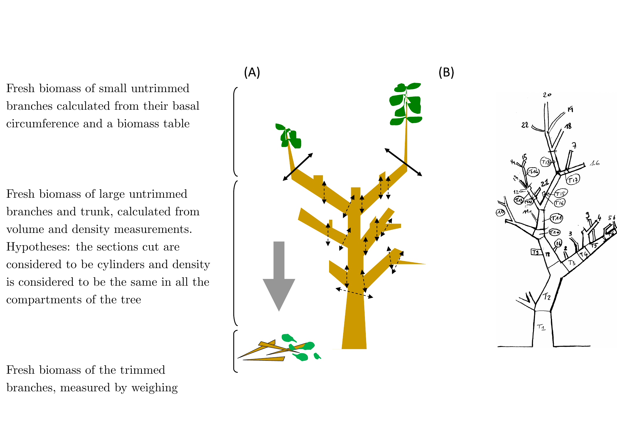
Figure 3.11: Determination of total fresh biomass. (A) Separation and measurement of trimmed and untrimmed biomass, (B) numbering of the sections and branches measured on a trimmed tree.
Trimmed fresh biomass
The branches may be trimmed in compliance with local practices (often using a machete). Use a measuring tape to determine the diameter at the base of each branch. Then separate the leaves from the trimmed branches. Determine (by weighing separately) the fresh biomass of the leaves from the trimmed branches (\(B_{\text{trimmed fresh leaf}}\)) and the fresh biomass of the wood from the trimmed branches (\(B_{\text{trimmed fresh wood}}\)). Suitable scales should be used for these weighing operations. If the leaves weigh less than 2 kg, they may be weighed using field-work electronic scales.
Take a random sample of the leaves from the trimmed branches. At least three samples of leaves from three different branches are generally required to constitute the aliquot. Measure its fresh weight (\(B_{\text{fresh leaf}}^{\text{aliquot}}\) in g). Take also an aliquot of the wood at random from the trimmed branches, without debarking. Measure its fresh mass (\(B_{\text{fresh wood}}^{\text{aliquot}}\) in g) in the field, immediately after cutting. Place these aliquots in numbered plastic bags and send to the laboratory. The fresh volume of the wood aliquot will be measured later in the lab (see § 3.2.2), and the value used to determine mean wood density \(\bar{\rho}\).
Untrimmed fresh biomass
Untrimmed biomass is measured indirectly as non-destructive. The different branches in the trimmed tree must first be numbered (Figure 3.11B). The small untrimmed branches must be processed differently from the large branches and the trunk (Figure 3.11A). For the small branches, only basal diameter needs to be measured. The biomass of these small untrimmed branches is estimated from the relationship between their basal diameter and their mass, as explained in section Calculating untrimmed biomass.
The biomass of the trunk and the large branches is estimated from measurements of volumes (\(V_i\) in cm3) and mean wood density (\(\bar{\rho}\) in g cm-3). The large branches and trunk should be divided virtually into sections that are then materialized by marking the tree. The volume \(V_i\) of each section \(i\) is obtained by measuring its diameter (or its circumference) and its length. Sections about one meter in length are preferable in order to consider diameter variations along the length of the trunk and branches.
3.2.2 In the laboratory
First, measure the volume (\(V_{\text{fresh wood}}^{\text{aliquot}}\)) of the wood aliquot taken from the trimmed compartments. This volume may be measured in different manners (Maniatis et al. 2011). That most commonly employed measures the volume of water displaced when the sample is immersed in water. The volume of water displaced may be measured using a graduated tube of suitable dimensions for the sample (Figure 3.12). Another method consists in cutting the sample into shapes whose volume may be accurately measured. This method requires precision tools and personnel trained in cutting wood.
Figure 3.12: Measuring sample volume by water displacement.
The wood and leaf aliquots should then be subject to the same laboratory measurements (oven drying, determination of dry weight, etc. ) as described in section 3.1.2.
3.2.3 Calculations
The dry biomass of the tree is obtained by the sum of the trimmed dry biomass and the untrimmed dry biomass: \[ B_{\text{dry}}=B_{\text{trimmed dry}}+B_{\text{untrimmed dry}} \]
Calculating trimmed biomass
From the fresh biomass \(B_{\text{fresh wood}}^{\text{aliquot}}\) of a wood aliquot and its dry biomass \(B_{\text{dry wood}}^{\text{aliquot}}\), calculate as above (see equation (3.2)) the moisture content of the wood (including bark): \[ \chi_{\text{wood}}=\frac{B^{\text{aliquot}}_{\text{dry wood}}}{B^{\text{aliquot}}_{\text{fres wood}}} \] Likewise, calculate the moisture content of the leaves from the fresh biomass \(B_{\text{fresh leaf}}^{\text{aliquot}}\) of the leaf aliquot and its dry biomass \(B_{\text{dry leaf}}^{\text{aliquot}}\): \[ \chi_{\text{leaf}}=\frac{B^{\text{aliquot}}_{\text{dry leaf}}}{B^{\text{aliquot}}_{\text{fresh leaf}}} \] Trimmed dry biomass can then be calculated: \[ B_{\text{trimmed dry}}=B_{\text{trimmed fresh wood}}\times \chi_{\text{wood}}+B_{\text{trimmed fresh leaf}}\times \chi_{\text{leaf}} \] where \(B_{\text{trimmed fresh leaf}}\) is the fresh biomass of the leaves stripped from the trimmed branches and \(B_{\text{trimmed fresh wood}}\) is the fresh biomass of the wood in the trimmed branches.
Calculating untrimmed biomass
Two calculations are required to calculate the dry biomass of the untrimmed part (i.e. that still standing): one for the small branches, the other for the large branches and the trunk. The untrimmed biomass is the sum of the two results: \[ B_{\text{untrimmed dry}}=B_{\text{untrimmed dry branch}} +B_{\text{dry section}} \] Each section \(i\) of the trunk and the large branches may be considered to be a cylinder of volume (Smalian’s formula): \[\begin{equation} V_i=\frac{\pi}{8}\ L_i\ (D_{1i}^2+D_{2i}^2)\tag{3.3} \end{equation}\] where \(V_i\) is the volume of the section \(i\), \(L_i\) its lenght, and \(D_{1i}\) and \(D_{2i}\) are the diameters of the two extremities of section \(i\). The truncated cone volume formula (see equation (3.1)) can also be used instead of the cylinder formula (3.3), but the difference between the results will be slight as the tapering over one meter is not very pronounced in trees.
The dry biomass of the large branches and trunk is the product of mean wood density and total volume of the large branches and trunk: \[\begin{equation} B_{\text{dry section}}=\bar{\rho}\times\sum_iV_i\tag{3.4} \end{equation}\] where the sum corresponds to all the sections in the large branches and the trunk (Figure 3.11B), and where mean wood density is calculated by: \[ \bar{\rho}=\frac{B_{\text{dry wood}}^{\text{aliquot}}} {V_{\text{fresh wood}}^{\text{aliquot}}} \] Care must be taken to use consistent measurement units. For example, if mean wood density \(\bar{\rho}\) in (3.4) is expressed in g cm-3, then volume \(V_i\) must be expressed in cm3, meaning that both length \(L_i\) and diameters \(D_{1i}\) and \(D_{2i}\) must also be expressed in cm. Biomass in this case is therefore expressed in g.
The dry biomass of the untrimmed small branches should then be calculated using a model between dry biomass and basal diameter. This model is established by following the same procedure as for the development of an allometric model (see chapters 4 to 7 herein). Power type equations are often used: \[ B_{\text{dry branch}}=a+bD^c \] where \(a\), \(b\) and \(c\) are model parameters and \(D\) branch basal diameter, but other regressions may be tested (see 5.1). Using a model of this type, the dry biomass of the untrimmed branches is: \[ B_{\text{untrimmed dry branch}}=\sum_j(a+bD_j^c) \] where the sum is all the untrimmed small branches and \(D_j\) is the basal diameter of the branch \(j\).
3.3 Partial weighings in the field
The third case we envisage is where the trees are too large to be weighed in their entirety by hand. We will illustrate this by developing an allometric equation to estimate the above-ground biomass of trees in a wet tropical forest based on destructive measurements. The method proposed must suit local circumstances and the resources available. And commercial value and the demand for timber are two other factors that must be taken into account when making measurements in forest concessions.
The trees selected must be felled using suitable practices. Variables such as total height, and height of any buttresses can be determined using a measuring tape. The tree’s architecture can then be analyzed (Figure 3.13). The proposed approach separates trees that can be weighed manually in the field (e.g. trees of diameter \(\leq20\) cm) from those requiring more substantial technical means (trees of diameter \(>20\) cm).
3.3.1 Trees less than 20 cm in diameter
The approach for trees of diameter \(\leq20\) cm, is similar to that described in the first example (§ 3.1). The branches and the trunk are first separated. The fresh biomass of the trunk (\(B_{\text{fresh trunk}}\)) and branches (\(B_{\text{fresh branch}}\), branch, wood and leaves together) is measured using appropriate scales. When measuring the biomass of the leaves, a limited number of branches should be selected at random for each individual. The leaves and the wood in this sample of branches should then be separated. The fresh biomass of the leaves (\(B_{\text{fresh leaf}}^{\text{sample}}\)) and the fresh biomass of the wood (\(B_{\text{fresh wood}}^{\text{sample}}\)) in this sample of branches should then be measured separately using appropriate scales. The foliage proportion of the branches must then be calculated: \[ \omega_{\text{leaf}}=\frac{B_{\text{fresh leaf}}^{\text{sample}}}{B_{\text{fresh leaf}}^{\text{sample}}+B_{\text{fresh wood}}^{\text{sample}}} \] The fresh biomass of the leaves (\(B_{\text{fresh leaf}}\)) and the wood (\(B_{\text{fresh wood}}\)) in the branches is then calculated based on this mean proportion of leaves: \[\begin{eqnarray*} B_{\text{fresh leaf}} &=& \omega_{\text{leaf}}\times B_{\text{fresh branch}} \\ B_{\text{fresh wood}} &=& (1-\omega_{\text{leaf}})\times B_{\text{fresh branch}} \end{eqnarray*}\] Aliquots of leaves and wood are then taken at different points along the branches and along the trunk. The fresh biomass (\(B_{\text{fresh leaf}}^{\text{aliquot}}\) and \(B_{\text{fresh wood}}^{\text{aliquot}}\)) of the aliquots must then be measured using electronic scales in the field. The aliquots must then be taken to the laboratory for drying and weighing in accordance with the same protocol as that described in the first example (§ 3.1.2). The oven-dry biomass (\(B_{\text{dry leaf}}^{\text{aliquot}}\) and \(B_{\text{oven-dry}}^{\text{aliquot}}\)) of the aliquots can then be used to calculate the water contents of the leaves and wood: \[ \chi_{\text{leaf}}=\frac{B_{\text{dry leaf}}^{\text{aliquot}}}{B_{\text{fresh leaf}}^{\text{aliquot}}},\qquad \chi_{\text{wood}}=\frac{B_{\text{dry wood}}^{\text{aliquot}}}{B_{\text{fresh wood}}^{\text{aliquot}}} \] Finally, the dry biomass of the leaves and wood is obtained from their fresh biomass and water contents calculated in the aliquots. The biomass of the wood is obtained by adding its fresh biomass to that of the branches and the trunk: \[\begin{eqnarray*} B_{\text{dry leaf}} &=& \chi_{\text{leaf}}\times B_{\text{fresh leaf}}\\ B_{\text{dry wood}} &=& \chi_{\text{wood}}\times(B_{\text{fresh wood}}+B_{\text{fresh trunk}}) \end{eqnarray*}\] Total dry mass is finally obtained by adding together the dry biomass of the leaves and the dry biomass of the wood: \[ B_{\text{dry}}=B_{\text{dry leaf}}+B_{\text{dry wood}} \]
3.3.2 Trees more than 20 cm in diameter
If a tree is very large, it possesses a very large quantity of branches and leaves, and it is impractical to separate the branches from the trunk. The alternative method proposed here therefore consists in processing the trunk and large branches (basal diameter more than 10 cm) differently from the small branches (basal diameter less than 10 cm). Whereas the large branches of basal diameter \(>10\) cm are made up only of wood, the small branches of diameter \(\leq10\) cm may also bear leaves. The large branches of basal diameter \(>10\) cm should be processed in the same manner as the trunk. The first step therefore consists in dividing the branches into sections. Whereas the biomass of the sections of diameter \(>10\) cm may be deduced from their measured volume (\(V_{\text{log},i}\)) and mean wood density (\(\bar{\rho}\)), that of the branches of basal diameter \(\leq10\) cm may be estimated using a regression between their basal diameter and the biomass they carry.
Measuring the volume of sections of diameter \(>10\) cm (trunk or branch)
Once the trunk and the branches of basal diameter \(>10\) cm have been divided into sections, the volume of each section can be calculated from their length and diameters (or circumferences) at the two extremities (\(D_{1i}\) and \(D_{2i}\)). A fixed length (e.g. two meters) may be used as the length of each section (photo 3.14A). A shorter section length than the fixed length must be used in some places where a fork prevents the log from assuming a cylindrical shape. The technician must record the length and diameters of each section before drawing a diagram of the tree’s architecture (Figure 3.13). This diagram is particularly useful for analyzing and interpreting the results.
Figure 3.13: Diagram showing the different sections of a tree used to calculate its volume.
Trees of diameter \(>20\) cm often have buttresses. The volume of the buttresses may be estimated by assuming that they correspond in shape to a pyramid, the upper ridge of which is a quarter ellipse (insert to Figure 3.13; Henry et al. 2010). For each buttress \(j\), we need to measure its height \(H_j\), its width \(l_j\) and its length \(L_j\) (insert to Figure 3.13).
Aliquots of wood must then be taken from the different sections of diameter \(>10\) cm (trunk, branches and any buttresses; photo 3.14B). These aliquots of fresh wood should be placed in tightly sealed bags and sent to the laboratory. In the laboratory, their volume (\(V_{\text{fresh wood}}^{\text{aliquot}}\)) should be measured in accordance with the protocol described in section 3.2.2. They should then be oven-dried and weighed as described in section 3.1.2. Their dry biomass (\(B_{\text{dry wood}}^{\text{aliquot}}\)) can be calculated from the results.
Figure 3.14: Measuring a large tree in the field: Left, measuring the volume of a tree of diameter > 20 cm; right, taking aliquots of wood from the trunk (photos: M. Henry).
Calculating the biomass of sections of diameter \(>10\) cm (trunk or branch)
As previously described (see equation (3.3)), the volume \(V_{\text{log},i}\) of the section \(i\) (trunk or branch of basal diameter \(>10\) cm) is calculated using Smalian’s formula: \[ V_{\text{log},i}=\frac{\pi\times L_i}{8}(D_{1i}^2+D_{2i}^2)\\ % \] where \(L_i\) is the length of the section \(i\), \(D_{1i}\) is the diameter at one of the extremities and \(D_{2i}\) is the diameter at the other. Given that its shape is that of a pyramid, a different formula is used to calculate the volume \(V_{\text{buttress},j}\) of the buttress \(j\): \[ V_{\text{buttress},j} = \left(1-\frac{\pi}{4}\right)\frac{L_jH_jl_j}{3} \] where \(l_j\) is the length of the buttress \(j\), \(L_j\) its length and \(H_j\) its height.
Mean wood density should then be calculated from the ovendry biomass and fresh volume of the wood aliquots: \[ \bar{\rho}=\frac{B_{\text{dry wood}}^{\text{aliquot}}} {V_{\text{fresh wood}}^{\text{aliquot}}} \] The cumulated dry biomass of the sections (trunk and branches of basal diameter \(>10\) cm) is therefore: \[ B_{\text{dry section}}=\bar{\rho}\times\sum_iV_{\text{log},i} \] where the sum corresponds to all the sections, whereas the dry biomass of the buttresses is: \[ B_{\text{dry buttress}}=\bar{\rho}\times\sum_jV_{\text{buttress},j} \] where the sum corresponds to all the buttresses. Alternatively, instead of using mean wood density, a specific density for each compartment (trunk, branches, buttresses) may also be employed. In this case mean wood density \(\bar{\rho}\) in the expressions above must be replaced by the specific density of the relevant compartment.
Measuring branches of diameter \(<10\) cm
The basal diameter of all branches of diameter \(\leq10\) cm, should now be measured and their dry biomass can be estimated from the regression between their basal diameter and the dry biomass they carry. This regression can be established from a sample of branches selected in the tree such as to represent the different basal diameter classes present. The leaves and the wood in this sample must now be separated. The fresh biomass of the leaves (\(B_{\text{fresh leaf},i}^{\text{sample}}\) in the branch \(i\)) and the fresh biomass of the wood (\(B_{\text{fresh wood},i}^{\text{sample}}\) in the branch \(i\)) are weighed separately in the field for each branch in the sample.
Some branches may be distorted and do not form a ramified architecture. In this case, the volume may be measured and the anomaly must be recorded in the field forms.
Aliquots of wood and leaves should then be taken and their fresh biomass (\(B_{\text{fresh wood}}^{\text{aliquot}}\) and \(B_{\text{fresh leaf}}^{\text{aliquot}}\)) determined immediately in the field. These aliquots should be placed in tightly sealed plastic bags and taken to the laboratory where they are oven-dried and weighed in accordance with the protocol described in section 3.1.2. Thus yields their ovendry biomass (\(B_{\text{dry wood}}^{\text{aliquot}}\) and \(B_{\text{dry leaf}}^{\text{aliquot}}\))
Calculating the biomass of branches of diameter \(<10\) cm
The fresh biomass of the aliquots serves to determine the water content of the leaves and wood: \[ \chi_{\text{leaf}}=\frac{B_{\text{dry leaf}}^{\text{aliquot}}}{B_{\text{fresh leaf}}^{\text{aliquot}}},\qquad \chi_{\text{wood}}=\frac{B_{\text{dry wood}}^{\text{aliquot}}}{B_{\text{fresh wood}}^{\text{aliquot}}} \] From this, and for each branch \(i\) of the sample of branches, may be determined the dry biomass of the leaves, the dry biomass of the wood, then the total dry biomass of branch \(i\): \[\begin{eqnarray*} B_{\text{dry leaf},i}^{\text{sample}} &=& \chi_{\text{leaf}}\times B_{\text{fresh leaf},i}^{\text{sample}} \\ B_{\text{dry wood},i}^{\text{sample}} &=& \chi_{\text{wood}}\times B_{\text{fresh wood},i}^{\text{sample}} \\ B_{\text{dry branch},i}^{\text{sample}} &=& B_{\text{dry leaf},i}^{\text{sample}}+B_{\text{dry wood},i}^{\text{sample}} \end{eqnarray*}\] In the same manner as in section Calculating untrimmed biomass, a biomass table for the branches can then be fitted to the data (\(B_{\text{dry branch},i}^{\text{sample}}\), \(D_i^{\text{sample}}\)), where \(D_i^{\text{sample}}\) is the basal diameter of the branch \(i\) of the sample. The biomass model for the branches may be established by following the same procedure as for the development of an allometric equation (see chapter 4 to 7 herein). To increase sample size, the model can be established based on all the branches measured for all the trees of the same species or by species functional group (Hawthorne 1995).
The branch biomass model established in this way can then be used to calculate the dry biomass of all branches of basal diameter \(\leq10\) cm: \[ B_{\text{dry branch}}=\sum_if(D_i) \] where the sum corresponds to all the branches of basal diameter \(\leq10\) cm, \(D_i\) is the basal diameter of the branch \(i\), and \(f\) is the biomass model that predicts the dry biomass of a branch on the basis of its basal diameter.
Calculating the biomass of the tree
The dry biomass of the tree may be obtained by summing the dry biomass of the sections (trunk and branches of basal diameter \(>10\) cm), dry biomass of the buttresses, and the dry biomass of the branches of diameter \(\leq10\) cm: \[ B_{\text{dry}}=B_{\text{dry sections}}+B_{\text{dry buttresses}}+B_{\text{dry branches}} \]
3.4 Measuring roots
It is far more difficult to determine root biomass than above-ground biomass. The methods we propose here are the results of campaigns conducted in different ecosystems and were compared in a study conducted in Congo (Levillain et al. 2011).
The first step, whatever the ecosystem, consists in drawing a Voronoi2 diagram around the selected tree. Figure 3.15 indicates the procedure employed: (i) draw the segments that link the selected tree to each of its neighbors; (ii) draw the bisectors for each segment, (iii) connect the bisectors one to another to bound a space around the tree; (iv) this space can then be divided into joined triangles, the area of each zone being easy to calculate when the length of all three sides (\(a\), \(b\) and \(c\)) is known: \[ A=\sqrt{p(p-2a)(p-2b)(p-2c)} \] where \(p=a+b+c\) is the triangle perimeter and \(A\) its area. Figure 3.16 illustrates this procedure for coconut plantations in Vanuatu (Navarro et al. 2008).
Figure 3.15: Method used to draw a Voronoi diagram and its subdivisions around a tree in any neighborhood situation.
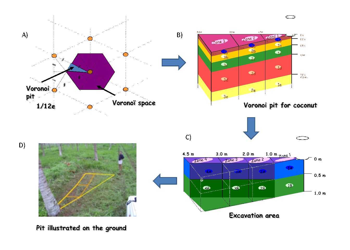
Figure 3.16: Typical Voronoi diagram used for root sampling in a coconut plantation in Vanuatu (photo: C. Jourdan). (A) Drawing the Voronoi space and choosing to work on \(1/12\)th of this space; (B) section through the pits dug; (C) protocol simplification given the variability observed in the first sample; (D) tracing the pit on the ground.
The space established in this manner is not a materialization of the tree’s “vital” space. It is simply a manner used to cut space into joined area to facilitate the sampling of below-ground biomass. The major hypothesis here is that the roots of other trees entering this space compensate for those of the selected tree leaving this space.
In the case of multispecific stands or agro-forest, it is sometimes impossible to separate the roots of the different species. In this case its would be very risky to construct individual models (root biomass related to the sampled tree), but root biomass estimations per hectare, without any distinction between species, are perfectly valid.
Sampling methods vary with root size. Levillain et al. (2011) conducted a study to compare different methods in the same tree (photo 3.17). They showed that the most profitable, in terms of cost-precision, was to sample the finest roots by coring, whereas medium-size roots require partial excavation and large roots total excavation from the Voronoi space.
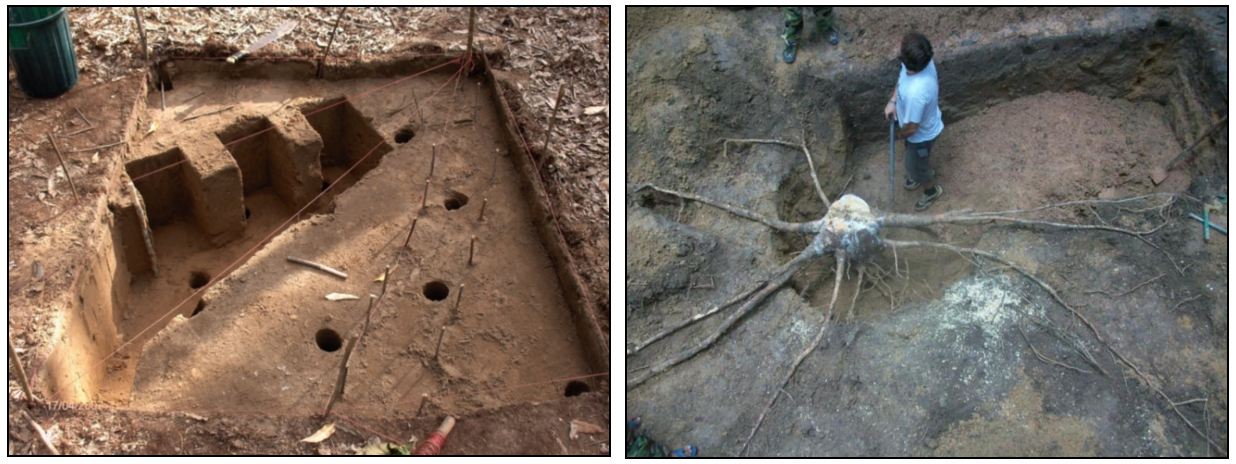
Figure 3.17: Left, superimposition of different sampling methods (cores, excavations by cubes, partial Voronoi excavation, total Voronoi excavation), from Levillain et al. (2011) (photo: C. Jourdan). Right, manual excavation of large roots in a rubber tree plantation in Thailand (photo: L. Saint-André).
The number of cores obtained and the size of the pit dug vary from one ecosystem to another. In Congo, in eucalyptus plantations, the optimum number of cores for 10 % precision is about 300 on the surface (0–10~cm) and about 100 for deeper roots (10–50 and 50–100~cm). Such a level of precision to a depth of 1~m requires 36 man-days. By contrast, if only 30 % precision is sought, this cuts sampling time by 75 %. This example clearly illustrates the usefulness of pre-sampling (see chapter 2) in order to evaluate the variability of the studied ecosystem then adapt the protocol to goals and desired precision.
Once the soil samples with the roots have been taken, the cores containing the fine roots can be sorted in the laboratory. On the other hand, given the volume and weight of the earth excavated, the medium-size and large roots must be sorted in the field. In the laboratory, the soil sample should first be washed through a filter and roots recovered either by flotation and/or by sieving. In the field, the samples should be sorted manually on tarpaulins. An air knife can be used on the large and medium-size roots to excavate the root system fully while preserving its architecture. This method, which is particularly advantageous in sandy soils, helps meet biomass and architecture goals but does require the presence of a mobile compressor (photo 3.18).
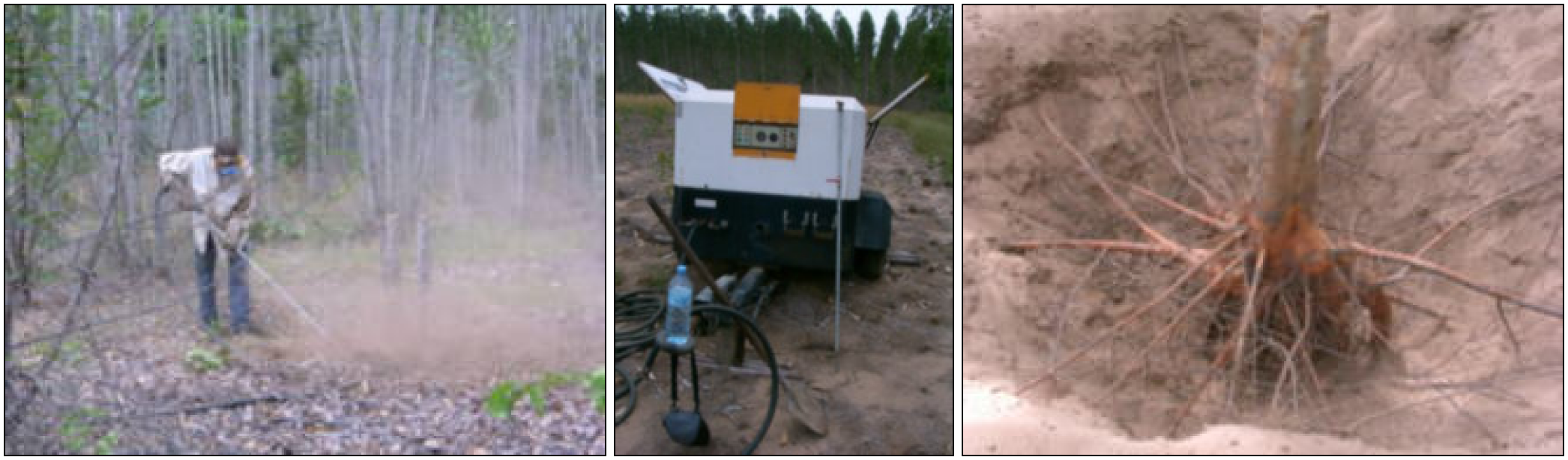
Figure 3.18: Air knife being used in Congo to extract the root systems (large and medium-size roots) of eucalyptus. Left, operator with protective equipment (dust, noise); middle, compressor and close up of the air pressure gauge (about 8 bars); right, the result (photos: C. Jourdan).
Once the roots have been sorted and harvested they should be dried in an oven using the same parameters as for above-ground biomass. The fine roots will require roughly the same drying time as for leaves, whereas the large and medium-size roots will need a drying time equivalent to that of branches.
Regarding the stump, a subsample should be taken, preferably vertically to better take account of wood density variations in this part of the tree. Here, the same procedures should be used as for the disks of the trunk.
The calculations then made are the same as for above-ground biomass.
3.5 Recommended equipment
3.5.1 Heavy machinery and vehicles
Cars, trucks, trailer: for transporting personnel, equipment and samples to/from the laboratory.
Quad bike (if possible): for transporting bulky equipment and samples in the field.
Digger for weighing brushwood bundles.
3.5.2 General equipment
Tool box with basic tools.
Plastic boxes (for storing and transporting materials — about 10).
Plastic bags (count one or two large bags per tree) to hold all the samples from a given tree and avoid water losses. Paper bags (count one per compartment and per tree) to hold samples immediately after they are taken. Ideally, these bags should be pre-labeled with tree and compartment number (which saves time in the field). But plan also to take a number of unmarked bags and a black, felt-tip pen (indelible ink) to make up for any mistakes made, or so that extra samples may be taken.
Large tarpaulins for the crown (either cut up for the branch bundles, or spread on the ground to recover leaves torn off the trees).
Labels (stapled onto the disks), staples and stapler; or fuschine pencil (but, if the samples are to be stored for later measurements of nutrient content, fuchsine should be avoided) (photo 3.19).
Cutters, machetes, axes, shears, saws (photo 3.19).
Iron frames for making bundling branches (photo 3.20) or alternatively bins of different sizes.
Power saws (ideally one power saw suitable for felling trees and another smaller more maneuverable power saw for limbing — photo 3.19).
Strong string for bundling the branches (given that this will be reused throughout the campaign, the knots should be undoable).
Very strong large bags (such as grain or sand bags — photo 3.21) for transporting the disks and field samples to vehicles (if these are parked some distance from the felling site).
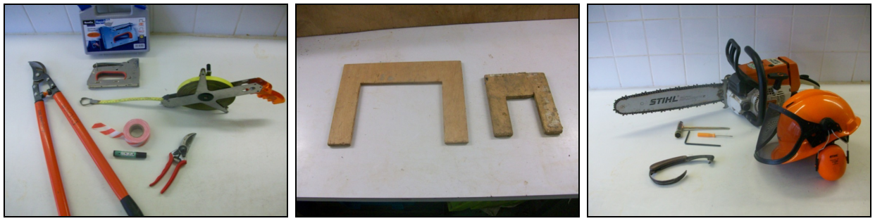
Figure 3.19: Field equipment. Left, equipment for cutting and labeling aliquots; middle, typical gauges for cutting branches; right, power saw and safety equipment (photo: A. Genet).
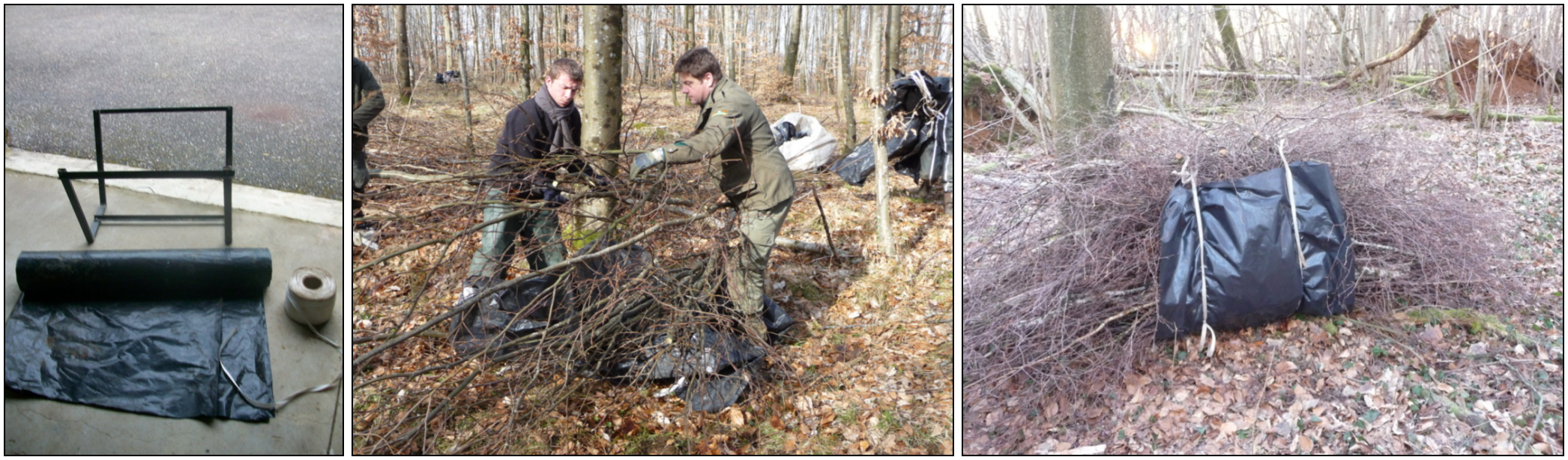
Figure 3.20: Bundling branches. Left, iron frame, tarpaulin and string for bundling branches (photo: A. Genet); middle, bundling branches in the field (photo: M. Rivoire); right, bundle ready for weighing (photo: M. Rivoire).
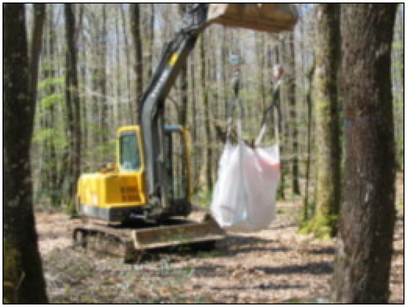
Figure 3.21: Transporting disks and aliquots in a sand or grain bag (photo: J.-F. Picard).
3.5.3 Computer-entering field data
Pocket PC (with battery charger and cables) or field record forms on waterproof paper or cardboard, if possible bound in notebooks with plasticized covers front and back.
Tree identification guide or key for wet tropical forest sites.
2B pencils, eraser, pencil sharpener.
Field scales (with 2 batteries and charger) for weighing samples (precise to within 1 g), ideally a full range of scales for different sample weights (a 1 or 2 m log may weigh several hundred kg, whereas the wood disks weigh from a few dozen g to several dozen kg). A digger will facilitate the field weighing of large logs. Straps should therefore be taken into the field to attach two scales to the bucket and self-blocking claws to attach the log.
Decameter to measure lengths along the trunk (stem profiles).
Tree calipers and girth tape to measure circumference.
Tree marking paint gun (for marking standing trees and the main stem in highly developed crowns).
Logger’s mark to indicate where disks should be cut (or marked with the paint gun).
3.5.4 Laboratory equipment
Ovens.
Graduated tubes of at least 500 ml.
Bark knife.
Secateurs.
Scales of a 2 to 2000 g capacity (precise to within 0.1 to 1 g).
Band saw.
3.6 Recommended field team composition
Felling team: one logger, two logging assistants, two persons to clear the area for felling. Count two days to fell 40 trees of 31 to 290~cm girth (mean: 140~cm). All the trees can be felled at the start of the campaign so that this team is freed for tree limbing. If team members are to be kept occupied, with no slack periods, about 10 trees per day (about 20~meters high, i.e. about 10 to 20 disks per tree) need to be ready for cross-cutting at the site.
Stem profiling team: two people (one anchor, one measurer). This team intervenes as soon as the tree has been felled, and therefore follows the felling team. In general, these two teams work in a fairly synchronized manner. The profiling team never has to wait for the felling team, except in very rare cases of felling problems (e.g. large stems, or stems imprisoned by other trees that need to be released).
Limbing team: three persons per processing unit. Each unit includes a power saw handler (with the small, maneuverable power saw) and two bundlers. These teams can be doubled or tripled depending on the size of the crown to be processed. As a rough guide: a tree with a breast-height girth of 200~cm will require three units; between girths of 80 and 200~cm the tree will require two units, and below a girth of 80~cm one unit will suffice. This rough guide includes the fact that the units must not hinder one another in their work. When three teams are working on the same tree, one should be positioned at the base, and should more upward along the length of the trunk. The two other teams should be positioned on each side of the main axis and should work from approximately the middle of the crown toward the top of the tree.
Logging team: this consists of one logger (cutting stems) and one person to label the disks. In general, the felling team fulfills this function. Once all the trees have been felled, the logger joins the logging team and the logging assistants bolster the limbing units.
Weighing team: three people (digger driver and two other persons to handle the logs and the branch bundles).
Branch sampling team: one or two people.
A Voronoi diagram (also called a Voronoi decomposition, a Voronoi partition or Voronoi polygons) is a special kind of decomposition of a metric space determined by distances to a specified family of objects, generally a set of points.↩︎