1 The foundations of biomass estimations
If we consider trees on a population scale, we see that the different dimensions of an individual are statistically related one with another (Gould 1966). This relation stems from the ontogenic development of individuals which is the same for all to within life history-related variability. For instance, the proportions between height and diameter, between crown height and diameter, between biomass and diameter follow rules that are the same for all trees, big or small, as long as they are growing under the same conditions (King 1996; Archibald and Bond 2003; Bohlman and O’Brien 2006; Dietze, Wolosin, and Clark 2008). This is the basic principle of allometry and can be used to predict a tree variable (typically its biomass) from another dimension (e.g. its diameter). An allometric equation is a formula that quantitatively formalizes this relationship. We will speak in this guide of volume, biomass and nutrient content models, respectively. Allometry also has another more restrictive definition: the proportionality relationship between relative increases in dimensions (Huxley 1924; Gayon 2000). If we call biomass \(B\) and diameter \(D\), this second definition means that there is a coefficient \(a\) such that: \[ \frac{\textsf{d}B}{B}=a\frac{\textsf{d}D}{D} \] which integrates to a power relationship: \(B=b\times D^a\). Using this restricted definition, an allometric equation is therefore synonymous with a power equation (White and Gould 1965). Parameter \(a\) gives the allometry coefficient (proportionality between relative increases), whereas parameter \(b\) indicates the proportionality between cumulated variables. It may be necessary to add a y-intercept to this relation that becomes \(B = c + bD^a\), where \(c\) is the biomass of an individual before it reaches the height at which diameter is measured (e.g. 1.30 m if \(D\) is measured at 1.30 m). The power relationship reflects the self-similarity idea of individuals during development (Gould 1971). It was this principle, and the “pipe model” (Shinozaki et al. 1964a, 1964b), that were used to develop an allometric scaling theory (West, Brown, and Enquist 1997, 1999; Enquist, Brown, and West 1998; Enquist et al. 1999). If we apply certain hypotheses covering biomechanical constraints, tree stability, and hydraulic resistance in the network of water-conducting cells, this theory predicts a power relationship with an exponent of \(a= 8/3 \approx 2.67\) between tree biomass and diameter. This relationship is of considerable interest as it is founded on physical principles and a mathematical representation of the cell networks within trees. It has nevertheless been the subject of much discussion, and has on occasion been accused of being too general in nature (Zianis and Mencuccini 2004; Zianis et al. 2005; Muller-Landau et al. 2006), even though it is possible to use other allometric coefficients depending on the biomechanical and hydraulic hypotheses selected (Enquist 2002).
Here in this guide we will adopt the broadest possible definition of allometry, i.e. a linear or non-linear correlation between increases in tree dimensions. The power relationship will therefore simply be considered as one allometric relationship amongst others. But whatever definition is adopted, allometry describes the ontogenic development of individuals, i.e. the growth of trees.
1.1 “Biology”: Eichhorn’s rule, site index, etc.
Tree growth is a complex biological phenomenon (Pretzsch 2009) resulting from the activity of buds (primary growth or axis elongation) and the cambium (secondary growth, or axis thickening). Tree growth is eminently variable as dependent upon the individual’s genetic heritage, its environment (soil, atmosphere), its developmental stage (tissue aging) and the actions of man (changes in the environment or in the tree itself through trimming or pruning).
Conventionally in biomass studies, trees are divided into homogeneous compartments: trunk wood, bark, live branches, dead branches, leaves, large and medium-size roots, and finally small roots. Biomass is a volume multiplied by a density, while nutrient content is a biomass multiplied by a concentration of nutrient. Volume, density and nutrient concentration change over time, not only in relation to the above-mentioned factors (see for example the review by Chave et al. 2009 on wood density) but also within trees: between compartments but also in relation to radial position (near the pith or the bark), and longitudinal position (near the soil or the crown), see for example regarding the concentrations of nutrient: Andrews and Siccama (1995); Colin-Belgrand, Ranger, and Bouchon (1996); Saint-André, Laclau, Deleporte, et al. (2002), Augusto et al. (2008); or for wood density: Guilley, Hervé, and Nepveu (2004); Bergès, Nepveu, and Franc (2008); Henry et al. (2010); Knapic, Louzada, and Pereira (2011). All this has implications for biomass and nutrient content equations, and this section therefore aims to underline a few important notions in forestry which will then be included in the process used to devise this guide’s models in “biological” terms (what factors can potentially cause variations?), rather than in purely mathematical terms (which is the best possible equation regardless of its likelihood of reflecting biological processes?). A combination of these two aims is ultimately this guide’s very purpose.
1.1.1 Even-aged, monospecific stands
This type of stand is characterized by a relatively homogeneous tree population: all are of the same age and most are of the same species. Tree growth in such stands has been the subject of much study (de Perthuis, 1788 in Batho and Garcı́a 2006) and the principles described below can be fairly universally applied (Assmann 1970; Dhôte 1991; Skovsgaard and Vanclay 2008; Pretzsch 2009; Garcı́a 2011). It is common practice to distinguish between the stand as a whole then the tree within the stand. This distinction dissociates the different factors that impact on trees growth: site fertility, overall pressure within the stand, and social status. Site fertility, in its broad sense, includes the soil’s capacity to nourish the trees (nutrients and water) and the area’s general climate (mean lighting, temperature and rainfall, usual recurrence of frost or drought, etc.). The pressure between trees in the stand can be assessed using a number of stand density indices. And the social status of each individual describes its capacity to mobilize resources in its immediate environment.
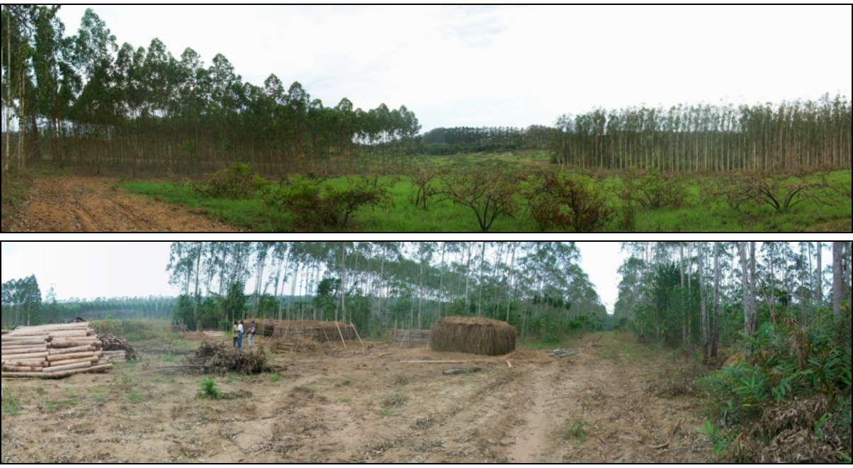
Figure 1.1: Eucalyptus plantation in the Republic of the Congo. Top is the Kissoko area, an illustration of savannah-plantation mosaics. Bottom is the Kondi area in operation, an illustration of the main destinations for eucalyptus wood (logs for paper pulp and charcoal production for the city of Pointe-Noire (photos: L. Saint-André).
Stand growth
The notion of production in forestry includes standing tree volume (or biomass) and all that has been subtracted from the stand over its lifecycle (by death or thinning). In general, this notion of production, as given in production tables and in most growth and yield models, does not include forest litter (fallen leaves, branches, bark) or root turnover. But in process-based models, and in studies aiming to estimate the carbon or mineral elements content of stands, the notion of production also includes the renewal of these organs. In the rest of this section we will consider production in its reduced definition.
The production of an even-aged, monospecific stand, for a given species in a given region and in a broad range of silvicultures (as long as the canopy is closed), is entirely determined by its mean height. This assertion is known as Eichhorn (1904), or Eichhorn’s extended rule when it considers dominant height instead of mean height (Decourt 1973). It means that the fertility of different sites in a given region modifies only the speed with which this relation is followed. Although the rule has been questioned (see Assmann 1970), the height growth of dominant trees (\(H_0\)) is still the main basic principle in most growth and models (e.g. Dhôte 1996; Garcı́a 2003, 2011; Saint-André et al. 2008; Skovsgaard and Vanclay 2008; Weiskittel et al. 2009). The principle is summarized by Alder (1980; in Pardé and Bouchon 1988) in the following sentence: “The height / age / fertility index relationship is key to predicting the growth of homogeneous stands. It is normally expressed in the form of a cluster of fertility plots”. Dominant height growth, as a first approximation, depends only on site fertility (in the broad sense, equivalent to the site index) and on stand age in most even-aged, monospecific, temperate or tropical ecosystems. This is the result of two main factors: because of their status, dominant trees are less sensitive that dominated trees to competition, and height growth is also less sensitive than diameter growth to silviculture (except a specific thinning regime). This means that dominant tree height growth is a more accurate indicator of site fertility than mean height or diameter growth. To achieve Eichhorn’s rule, it is then necessary to couple basal area (or volume) growth and dominant tree height growth. This relationship is also stable for a given species and a given region in a broad range of silvicultures (as a first approximation provided that the canopy is sufficiently dense). An example for beech in France is given by Dhôte (1996).
But there are a few examples where the strict relationship of \(H_0 = f\) (age and fertility) is invalid: the Laricio pine in central France (Meredieu, Perret, and Dreyfus 2003) and eucalyptus in the Republic of Congo (Saint-André, Laclau, Bouillet, et al. 2002). In both cases dominant tree height growth also depends on stand density. The underlying hypothesis is based on poor soil fertility that means strong competition for access to water and mineral resources, even for dominant trees. Over the last few years, a “date” effect has also been clearly shown, both for this relationship and that linking basal area growth and dominant tree height growth, due to global changes (see for example Bontemps, Hervé, and Dhôte 2009; Bontemps et al. 2011; Charru et al. 2010).
In short, even though it is in dispute and is not necessarily as invariable as was hoped, this first “rule” is nevertheless important as it can be used, in so-called parameterized biomass tables, to introduce the notion of fertility through dominant tree age and height in inventoried stands (and incidentally density) and thereby increase the generic nature of the equations constructed.
Tree growth in a stand
When volume or biomass growth is obtained for an entire stand, efforts must be made to distribute this between the different trees. The relationships employed for individual diameter growth are often of the potential \(\times\) reducer type, where the potential is given by basal area growth and / or dominant tree growth, and the reducers depend on (i) a density index and (ii) the tree’s social status. A density index may simply be stand density, but researchers have developed other indices such as the Hart-Becking spacing index, based on the growth of trees outside the stand (free growth), or the Reinecke density index (RDI), based on the self-thinning rule (tree growth in a highly dense stand). Both of these have the advantage of being less dependent upon stand age than on density itself (see Shaw 2006 or more generally the literature review by @vanclay09). The social status of trees is generally expressed by ratios such as \(H/H_0\) or \(D/D_0\) (where \(D\) is tree diameter at breast height, \(H\) its height and \(D_0\) the diameter at breast height (dbh) of the dominant tree in the stand), but other relationships may also be used. For example, Dhôte (1990), Saint-André, Laclau, Bouillet, et al. (2002) and more recently Cavaignac et al. (2012) used a piecewise linear model to model tree diameter growth: below a certain circumference threshold, trees are overtopped and no longer grow; above the threshold their growth shows a linear relationship with tree circumference. This relationship clearly expresses the fact that dominant trees grow more than dominated trees. The threshold and slope of the relationship change with stand age and silviculture treatments (thinning). Although height growth may also be estimated using potential \(\times\) reducer relationships, modelers generally prefer height-circumference relationships (Soares and Tomé 2002). These relationships are saturated (the asymptote is the height of the dominant tree in the stand) and curvilinear. This relationship’s parameters also change with age and silviculture treatment (Deleuze, Blaudez, and Hervé 1996).
These two other relationships give the dimension of each tree in stands, and in particular it should be underlined that the density and competition (social status) indices that largely determine the individual growth of trees in stands are factors that can also be integrated into biomass tables. Interesting variables from this standpoint are stand density, the Hart-Becking spacing index, the RDI, then — on an individual scale — the slenderness ratio (\(H/D\)), tree robustness (\(D^{1/2}/H\) — Vallet et al. 2006; Gomat et al. 2011), or its social status (\(H/H_0\) or \(D/D_0\)).
Biomass distribution in the tree
Finally, now that stand biomass has been distributed between the trees, we need to attribute it to each compartment in each tree and distribute it along the axes. Regarding the trunk, Pessler’s rule is usually employed (or for ecophysiologists its equivalent given by the pipe model described by Shinozaki et al. 1964a, 1964b): (i) ring cross-sectionnal area increases in a linear manner from the top of the tree to the functional base of the crown; (ii) it is then constant from the base of the crown to the base of the tree. This means that as the tree grows its trunk becomes increasingly cylindrical as the growth rings are wider apart near the crown than at the base. Pressler’s rule, however, does not express the mean distribution of wood along the tree (Saint-André et al. 1999) since ring mark area in dominant trees may continue to increase beneath the crown, and in dominated / overtopped trees it may greatly decrease. In extreme cases the growth ring may not be complete at the base of the tree, or may even be entirely missing as for example in the beech (Nicolini, Chanson, and Bonne 2001). Also, any action on the crown (high or low densities, thinning, trimming) will have an impact on the distribution of annual growth rings and therefore on the shape of the trunk (see the review by Larson 1963, or the examples given by @valinger92; Ikonen et al. 2006). Wood density is also different at the top and base of the tree (young wood near the crown, high proportion of adult wood toward the base — Burdon et al. 2004) but it may also vary according to the condition of the tree’s growth (changes in proportion between early and late wood, or changes in cell structure and properties, see Guilley, Hervé, and Nepveu 2004; Bouriaud et al. 2005; Bergès, Nepveu, and Franc 2008 for some recent papers). Therefore, the biomass of different trunks of the same dimensions (height, dbh, age) may be the same or different depending on the conditions of tree growth. An increase in trunk volume may be accompanied by a decrease in its wood density (as typically in softwoods), and does not therefore cause a major difference in trunk biomass. Regarding branches and leaves, their biomass is greatly dependent upon tree architecture and therefore on stand density: considering trees of equal dimensions (height, dbh and age), those growing in open stands will have more branches and leaves than those growing in dense stands. The major issue, therefore, in current research on biomass consists in identifying the part of the biomass related to the tree’s intrinsic development (ontogenics) and that related to environmental factors (Thornley 1972; Bloom, Chapin, and Mooney 1985; West, Brown, and Enquist 1999; McCarthy and Enquist 2007; Savage, Deeds, and Fontana 2008; Genet et al. 2011; Gourlet-Fleury et al. 2011). And the biomass of the roots depends on the biome, on above-ground biomass, development stage and growing conditions (see for example Jackson et al. 1996; Cairns et al. 1997; Tateno, Hishi, and Takeda 2004; Mokany, Raison, and Prokushkin 2006).
What emerges from these notions is that growing conditions have an impact not only on the overall amount of biomass produced, but also on its distribution within the tree (above-ground / below-ground proportion, ring stacking, etc.). These potential variations must therefore be taken into account when sampling (particularly for crosscutting trunks and taking different aliquots), but also when constructing volume/biomass tables such that they reflect correctly the different above-ground / below-ground; trunk / branch; leaves / small roots biomass ratios resulting from different growing conditions.
1.1.2 Uneven-aged and/or multispecific stands
The notions described above are also valid for multispecific and uneven-aged stands, but in most cases their translation into equations is impossible in the previous form (Peng 2000). For example, the notion of dominant height is difficult to quantify for irregular and / or multispecific stands (should we determine a dominant height considering all the trees? Or species by species?). Likewise, what does basal area growth mean for a very irregular stand as can be found in wet tropical forests? And finally, how can we deal with the fact that tree age is often inaccessible (Tomé et al. 2006)? The growth models developed for these stands therefore more finely break down the different scales (biomass produced on the stand scale, distribution between trees and allocation within trees) than do those developed for regular stands. These models may be divided into three types: (1) matrix population models; (2) individual-based models that in general depend on the distances between trees; (3) gap models (see the different reviews by Vanclay 1994; Franc, Gourlet-Fleury, and Picard 2000; Porté and Bartelink 2002). Matrix population models divide trees into functional groups (with a common growth strategy) and into classes of homogeneous dimensions (generally diameter) then apply a system of matrices that include recruitment, mortality and the transition of individuals from one group to another (see for example Eyre and Zillgitt 1950; Favrichon 1998; Namaalwa, Eid, and Sankhayan 2005; Picard et al. 2008). In individual-based models, the tree population is generally mapped and the growth of a given tree depends on its neighbors (see for example Gourlet-Fleury and Houllier 2000 for a model in tropical forest, or @courbaud01 for a model in temperate forest). But, like for the models developed for regular stands, some individual-based models are independent of distances (for example Calama et al. 2008; Pukkala, Lähde, and Laiho 2009; Vallet and Pérot 2011; Dreyfus 2012) and even intermediate models (see Picard and Franc 2001; Verzelen, Picard, and Gourlet-Fleury 2006; Perot et al. 2010). Finally, in gap models, the forest is represented by a set of cells at different stages of the silvigenetic cycle. Here, tree recruitment and mortality are simulated stochastically while tree growth follows identical rules to those of distance-independent, individual-based models (see a review in Porté and Bartelink 2002).
The fact that these stands are more complicated to translate into equations does not in any way detract from the principles mentioned above for the construction of volume, biomass or nutrient content tables: (i) fertility is introduced to broaden the range over which the biomass tables are valid; (ii) density indices are used to take account of the degree of competition between trees; and (iii) social status is taken into account in addition to tree basic characteristics (height, diameter).
The development of volume/biomass tables for multispecific forests faces a number of constraints in addition to those facing tables for monospecific forests: conception of suitable sampling (which species? how can species be divided into so-called functional groups?), access to the field (above all in tropical forests where stands are often located in protected area where felling is highly regulated or even prohibited for certain species).
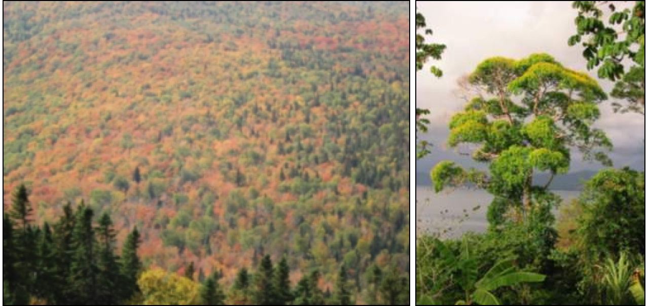
Figure 1.2: Heterogeneous stands. On the left, multispecific stands on Mont Saint-Anne in Quebec; on the right, multispecific, uneven-aged stands in Costa-Rica (photo: B. Locatelli).
1.2 Selecting a method
1.2.1 Estimating the biomass of a biome
There is no single method for estimating biomass stocks, but a number of methods depending on the scale considered (Gibbs et al. 2007). On a national or larger scale, mean values per biome are usually employed (FAO 2006): the amount of biomass is estimated by multiplying the surface area of each biome by the mean amount of biomass per unit surface area of this biome. And mean amounts per biome are estimated from measurements made on a smaller scale. Biomass on national to landscape scales can be estimated by remote sensing. Regardless of whether this uses satellite-borne optical sensors (Landsat, MODIS), high resolution satellite images (Ikonos, QuickBird), low resolution aerial photographs, satellite-borne radar or microwave sensors (ERS, JERS, Envisat, PALSAR), or laser sensors (Lidar), all these methods assume that field measurements are available to adjust biomass-predicting models to remote sensing observations. When dealing with satellite-borne optical sensors, field data are necessary to calibrate the relationship between biomass and satellite vegetation indices (NDVI, NDFI, AVI, GVI, etc.) (Dong et al. 2003; Saatchi et al. 2007). High-resolution images and aerial photographs provide information on tree crown size and height, and field data are then necessary to relate this information to biomass (for example Bradley 1988; Holmgren, Masakha, and Sjöholm 1994; St.-Onge, Hu, and Vega 2008; Gonzalez et al. 2010). The same applies to Lidar information on the vertical structure of forests, and to radar and microwave information on the vertical distribution of plant water (for example Lefsky et al. 2002; Patenaude et al. 2004). But remote sensing-based methods have their limitations in terms of providing precise biomass measurements (particularly surface areas) and differentiating forest types due to the technical, financial and human resources available. They are also hindered by cloud cover and are susceptible to saturated signals for certain vegetation types.
Therefore, biomass estimation methods on a landscape or greater scale rely on field measurements taken between the landscape and plot scales. Biomass estimations on this scale are based on forest inventory data: inventory of a sample of trees if the area is large, or otherwise a full inventory (particularly in permanent plots of a few hectares). On a smaller scale, individual biomass measurements may be taken by weighing trees and understorey vegetation.
1.2.2 Estimating the biomass of a forest or a set of forests
Estimations of forest biomass or nutrient content based on forest inventories require:
- an exhaustive or statistical inventory of the trees growing;
- models to evaluate carbon stocks from the dimensions of the individuals measured;
- an evaluation of the biomass contained in the necromass (standing dead wood) and in understorey vegetation.
In this guide we focus on the second aspect even though an inventory and quantitative evaluation of the understorey is not necessarily easy to obtain, particularly in highly mixed forests.
Two main methods based on inventory data may be employed to estimate tree carbon or mineral element stocks (MacDicken 1997; Hairiah et al. 2001; AGO 2002; Ponce-Hernandez, Koohafkan, and Antoine 2004; Monreal et al. 2005; Pearson and Brown 2005; Dietz and Kuyah 2011): (1) use of biomass/nutrient content tables: this solution is often adopted as it rapidly yields the carbon or nutrient content of a plot at a given time point. In general, all the different (above-ground, below-ground, ground litter, etc.) compartments of the ecosystem are considered. Trees are specifically felled for these operations. The compartments (cross cuts) may vary depending on application and the field of interest (see chapter 3). (2) Use of models to estimate successively tree volume, wood density and nutrient content. This method has the advantage of dissociating the different components, making it possible to analyze the effect of age and growing conditions independently on one or another of the components. In general, only the trunk can be modeled in detail (between and within rings). The biomass of the other compartments is estimated from volume expansion factors, mean wood density measurements and nutrient concentration. In all cases these models call upon one and the same model type that indifferently groups together “volume tables, biomass tables, nutrient content tables, etc.” and which is described here in this guide.
Biomass and nutrient content tables are closely related to volume tables that have been the subject of much study for nearly two centuries. The first tables were published by Cotta (1804; in Bouchon 1974) for beech (Fagus sylvatica). The principle employed is to link a variable that is difficult to measure (e.g. the volume of a tree, its mass, or its mineral elements content) to variables that are easier to determine, e.g. tree diameter at breast height (DBH) or height. If both characteristics are used, we speak of a double-entry table; if only DBH is used, we speak of a single-entry table. In general, close correlations are obtained and the polynomial, logarithmic and power functions are those most widely used. For more details, readers may see the reviews by Bouchon (1974); Hitchcock and McDonnell (1979); Pardé (1980); Cailliez (1980); Pardé and Bouchon (1988), and more recently by Parresol (1999); Parresol (2001).
These functions are relatively simple but have three major snags. First, they are not particularly generic: if we change species or stray outside the calibration range, the equations must be used with caution. The chapter on sampling gives a few pointers on how to mitigate this problem. The key principle is to cover as best as possible the variability of the quantities studied.
The second snag with these functions lies in the very nature of the data processed (volumes, masses, nutrient content). In particular, problems of heteroscedasticity may arise (i.e. non homogeneous variance in biomasses in relation to the regressor). This has little impact on the value of the estimated parameters: the greater the number of trees sampled, the more rapid the convergence toward real parameter values (Kelly and Beltz 1987). But everything concerning the confidence interval of the estimations is affected:
- the variance of the estimated parameters is not minimal;
- this variance is biased; and
- residual variance is poorly estimated (Cunia 1964; Parresol 1993; Gregoire and Dyer 1989).
If no efforts are made to correct these heteroscedasticity problems, this has little impact on the mean biomass or volume values estimated. By contrast, these corrections are indispensable if we are to obtain correct confidence intervals around these predictions. Two methods are often put forward to correct these heteroscedasticity problems: the first consists in weighting (for instance by the inverse of the diameter or the squared diameter), but here everything depends on the weighting function and in particular on the power applied. The second consists in taking the logarithm of the terms in the equation, but here the simulated values need to be corrected to ensure that the estimated values return to a normal distribution (Duan 1983; Taylor 1986). Also, it may well happen that the log transformation does not result in a linear model (Návar, Méndez, and Dale 2002; Saint-André et al. 2005).
The third snag is due to the additivity of the equations. Biomass measurements, then the fitting of functions, are often made compartment by compartment. The relations are not immediately additive, and a desired property of the equations system is that the sum of the biomass predictions made compartment by compartment equals the total biomass predicted for the tree (see Kozak 1970; Reed and Green 1985; Návar, Méndez, and Dale 2002). Three solutions are in general suggested (Parresol 1999):
total biomass is calculated by summing the compartment by compartment biomasses, and the variance of this estimation uses the variances calculated for each compartment and the covariances calculated two by two;
additivity is ensured by using the same regressors and the same weights for all the functions, with the parameters of the total biomass function being the sum of the parameters obtained for each compartment;
the models are different compartment by compartment but are fitted jointly, and additivity is obtained by constraints on the parameters.
Each method has its advantages and disadvantages. Here in this guide we will fit a model for each compartment and a model for total biomass, while checking that additivity is respected. Concrete examples (dubbed “red lines”) will be used throughout this guide as illustrations. These are based on datasets obtained during studies conducted in a natural wet tropical forest in Ghana (Henry et al. 2010).
1.2.3 Measuring the biomass of a tree
Biomass tables create a link between actual individual biomass measurements and biomass estimations in the field based on inventory data. Weighing trees to measure their biomass is therefore an integral part of the approach used to construct allometric equations, and a large part of this guide is therefore devoted to describing this operation. Although the general principles described in chapter 3 (tree segmentation into compartments of homogenous dry weight density, measurement of dry matter / fresh volume ratios in aliquots, and application of a simple rule of three) should yield a biomass estimation for any type of woody plant, this guide will not address all the special cases. Plants that are not trees but potentially have the stature of trees (bamboo, rattan, palms, tree ferns, Musaceae, Pandanus spp., etc.) are considered as exceptions.
Plants that use trees as supports for their growth (epiphytes, parasitic plants, climbers, etc.) are another special case (Putz 1983; Gerwing and Farias 2000; Gerwing et al. 2006; Gehring, Park, and Denich 2004; Schnitzer, DeWalt, and Chave 2006; Schnitzer, Rutishauser, and Aguilar 2008). Their biomass should be dissociated from that of their host.
Finally, hollow trees, and trees whose trunks are shaped very differently from a cylinder (e.g. Swartzia polyphylla DC.), strangler fig, etc., are all exceptions to which biomass tables cannot be applied without specific adjustments (Nogueira, Nelson, and Fearnside 2006).